Prelims

Aeronautical

Engineer’s

Data Book

Clifford Matthews BSc, CEng, MBA, FIMechE

OXFORD AUCKLAND BOSTON JOHANNESBURG

MELBOURNE NEW DELHI

Butterworth-Heineman

Linacre House, Jordan Hill, Oxford OX2 8DP

225 Wildwood Avenue, Woburn, MA 01801-2041

A division of Reed Educational and Professional Publishing Ltd

A member of the Reed Elsevier plc group

First published 2002

may be reproduced in any material form (including

photocopying or storing in any medium by electronic

means and whether or not transiently or incidentally

to some other use of this publication) without the

written permission of the copyright holder except

in accordance with the provisions of the Copyright,

Designs and Patents Act 1988 or under the terms of a

licence issued by the Copyright Licensing Agency Ltd,

90 Tottenham Court Road, London, England W1P 9HE.

Applications for the copyright holder’s written permission

to reproduce any part of this publication should be addressed

to the publishers

British Library Cataloguing in Publication Data

Matthews, Clifford

Aeronautical engineer’s data book

1. Aerospace engineering–Handbooks, manuals, etc.

I. Title

629.1’3

Library of Congress Cataloguing in Publication Data

Matthews, Clifford.

Aeronautical engineer’s data book / Clifford Matthews.

p. cm.

Includes index.

ISBN 0 7506 5125 3

1. Aeronautics–Handbooks, Manuals, etc. I. Title.

TL570.M34 2001

629.13'002'12–dc21 2001037429

ISBN 0 7506 5125 3

Composition by Scribe Design, Gillingham, Kent, UK

Printed and bound by A. Rowe Ltd,

Chippenham and Reading, UK

Contents

Acknowledgements vii

Preface ix

Disclaimer x

1 Important Regulations and Directives 1

2 Fundamental Dimensions and Units 6

2.1 The Greek alphabet 6

2.2 Units systems 7

2.3 Conversions 8

2.4 Consistency of units 20

2.5 Foolproof conversions: using unity

brackets 21

2.6 Imperial–metric conversions 22

2.7 Dimensional analysis 22

2.8 Essential mathematics 25

2.9 Useful references and standards 47

3 Symbols and Notations 49

3.1 Parameters and constants 49

3.2 Weights of gases 49

3.3 Densities of liquids at 0°C 50

3.4 Notation: aerodynamics and fluid

mechanics 50

3.5 The International Standard

Atmosphere (ISA) 56

4 Aeronautical Definitions 66

4.1 Forces and moments 66

4.2 Basic aircraft terminology 70

4.3 Helicopter terminology 71

4.4 Common aviation terms 72

4.5 Airspace terms 75

5 Basic Fluid Mechanics 76

5.1 Basic properties 76

5.2 Flow equations 79

iv Contents

5.3 Flow regimes 86

5.4 Boundary layers 88

5.5 Isentropic flow 89

5.6 Compressible 1D flow 90

5.7 Normal shock waves 91

5.8 Axisymmetric flow 93

5.9 Drag coefficients 94

6 Basic Aerodynamics 96

6.1 General airfoil theory 96

6.2 Airfoil coefficients 96

6.3 Pressure distributions 98

6.4 Aerodynamic centre 100

6.5 Centre of pressure 101

6.6 Supersonic conditions 102

6.7 Wing loading: semi-ellipse

assumption 103

7 Principles of Flight Dynamics 106

7.1 Flight dynamics – conceptual

breakdown 106

7.2 Axes notation 106

7.3 The generalized force equations 110

7.4 The generalized moment equations 110

7.5 Non-linear equations of motion 111

7.6 The linearized equations of motion 111

7.7 Stability 114

8 Principles of Propulsion 115

8.1 Propellers 115

8.3 Engine data lists 126

8.4 Aero engine terminology 126

8.5 Power ratings 129

9 Aircraft Performance 132

8.2 The gas turbine engine: general

principles 118

9.1 Aircraft roles and operational profile 132

9.2 Aircraft range and endurance 136

9.3 Aircraft design studies 138

9.4 Aircraft noise 140

9.5 Aircraft emissions 144

10 Aircraft Design and Construction 145

10.1 Basic design configuration 145

10.2 Materials of construction 164

10.3 Helicopter design 165

10.4 Helicopter design studies 168

v Contents

11 Airport Design and Compatibility 173

11.1 Basics of airport design 173

11.2 Runway pavements 196

11.3 Airport traffic data 197

11.4 FAA-AAS airport documents 197

11.5 Worldwide airport geographical data 205

11.6 Airport reference sources and

bibliography 205

12 Basic Mechanical Design 215

12.1 Engineering abbreviations 215

12.2 Preferred numbers and preferred sizes 215

12.3 Datums and tolerances – principles 217

12.4 Toleranced dimensions 218

12.5 Limits and fits 223

12.6 Surface finish 227

12.7 Computer aided engineering 224

13 Reference Sources 235

13.1 Websites 235

13.2 Fluid mechanics and aerodynamics 235

13.3 Manufacturing/materials/structures 235

13.4 Aircraft sizing/multidisciplinary design 240

13.5 Helicopter technology 240

13.6 Flying wings 240

13.7 Noise 241

13.8 Landing gear 241

13.9 Airport operations 241

13.10Propulsion 242

Appendix 1 Aerodynamic stability and control

derivatives 243

Appendix 2 Aircraft response transfer

functions 245

Appendix 3

Approximate expressions for

dimensionless aerodynamic

stability and control derivatives 247

Appendix 4 Compressible flow tables 253

Appendix 5 Shock wave data 261

Index 269

Preface

The objective of this Aeronautical Engineer’s

Data book is to provide a concise and useful

source of up-to-date information for the

student or practising aeronautical engineer.

Despite the proliferation of specialized infor-

mation sources, there is still a need for basic

data on established engineering rules, conver-

sions, modern aircraft and engines to be avail-

able in an easily assimilated format.

An aeronautical engineer cannot afford to

ignore the importance of engineering data and

rules. Basic theoretical principles underlie the

design of all the hardware of aeronautics. The

practical processes of fluid mechanics, aircraft

design, material choice, and basic engineering

design form the foundation of the subject.

Technical standards, directives and regulations

are also important – they represent accumu-

lated knowledge and form invaluable guide-

lines for the industry.

The purpose of the book is to provide a

basic set of technical data that you will find

useful. It is divided into 13 sections, each

containing specific ‘discipline’ information.

Units and conversions are covered in Section

2; a mixture of metric and imperial units are

still in use in the aeronautical industry. Infor-

mation on FAA regulations is summarized in

Section 1 – these develop rapidly and affect us

all. The book contains cross-references to

other standards systems and data sources. You

will find these essential if you need to find

more detailed information on a particular

subject. There is always a limit to the amount

viii Preface

of information that you can carry with you –

the secret is knowing where to look for the

rest.

More and more engineering information is

now available in electronic form and many

engineering students now use the Internet as

their first source of reference information for

technical information. This new

Aeronautical

Engineer’s Data Book contains details of a

wide range of engineering-related websites,

including general ‘gateway’ sites such as the

Edinburgh Engineering Virtual Library

(EEVL) which contains links to tens of

thousands of others containing technical infor-

mation, product/company data and aeronauti-

cal-related technical journals and newsgroups.

You will find various pages in the book

contain ‘quick guidelines’ and ‘rules of thumb’.

Don’t expect these all to have robust theoret-

ical backing – they are included simply

because I have found that they work

. I have

tried to make this book a practical source of

aeronautics-related technical information that

you can use in the day-to-day activities of an

aeronautical career.

Finally, it is important that the content of

this data book continues to reflect the infor-

mation that is needed and used by student and

experienced engineers. If you have any sugges-

tions for future content (or indeed observations

or comment on the existing content) please

submit them to me at the following e-mail

address: [email protected]

Clifford Matthews

Acknowledgements

Special thanks are due to Stephanie Evans,

Sarah Pask and John King for their excellent

work in typing and proof reading this book.

Disclaimer

This book is intended to assist engineers and

designers in understanding and fulfilling their

obligations and responsibilities. All interpreta-

tion contained in this publication – concerning

technical, regulatory and design information

and data, unless specifically otherwise identi-

fied, carries no authority. The information

given here is not intended to be used for the

design, manufacture, repair, inspection or

certification of aircraft systems and equipment,

whether or not that equipment is subject to

design codes and statutory requirements.

Engineers and designers dealing with aircraft

design and manufacture should not use the

information in this book to demonstrate

compliance with any code, standard or regula-

tory requirement. While great care has been

taken in the preparation of this publication,

neither the author nor the publishers do

warrant, guarantee, or make any representa-

tion regarding the use of this publication in

terms of correctness, accuracy, reliability,

currentness, comprehensiveness, or otherwise.

Neither the publisher, author, nor anyone, nor

anybody who has been involved in the

creation, production, or delivery of this

product shall be liable for any direct, indirect,

consequential, or incidental damages arising

from its use.

Section 1

Important regulations and

directives

A fundamental body of information is

contained in the US Federal Aviation Regula-

tions (FAR). A general index is shown below:

Federal Aviation Regulations

Chapters I and III

Subchapter A – definitions and

abbreviations

Part 1: Definitions and abbreviations

Subchapter B – procedural rules

Part 11: General rule-making procedures

Part 13:

Investigative and enforcement

procedures

Part 14: Rules implementing the Equal

Access to Justice Act of 1980

Part 15: Administrative claims under

Federal Tort Claims Act

Part 16: Rules of practice for federally-

assisted airport enforcement

proceedings

Part 17: Procedures for protests and

contracts disputes

Subchapter C – aircraft

Part 21: Certification procedures for

products and parts

Part 23: Airworthiness standards: normal,

utility, acrobatic, and commuter

category airplanes

Part 25: Airworthiness standards: transport

category airplanes

2 Aeronautical Engineer’s Data Book

Part 27: Airworthiness standards: normal

category rotorcraft

Part 29: Airworthiness standards: transport

category rotorcraft

Part 31: Airworthiness standards: manned

free balloons

Part 33: Airworthiness standards: aircraft

engines

Part 34: Fuel venting and exhaust emission

requirements for turbine engine

powered airplanes

Part 35: Airworthiness standards:

propellers

Part 36: Noise standards: aircraft type and

airworthiness certification

Part 39: Airworthiness directives

Part 43: Maintenance, preventive

maintenance, rebuilding, and

alteration

Part 45: Identification and registration

marking

Part 47: Aircraft registration

Part 49: Recording of aircraft titles and

security documents

Subchapter D – airmen

Part 61: Certification: pilots and flight

instructors

Part 63: Certification: flight crewmembers

other than pilots

Part 65: Certification: airmen other than

flight crewmembers

Part 67: Medical standards and certification

Subchapter E – airspace

Part 71: Designation of class a, class b,

class c, class d, and class e

airspace areas; airways; routes; and

reporting points

Part 73: Special use airspace

Part 77: Objects affecting navigable

airspace

Subchapter F – air traffic and

3 Important regulations and directives

general operation rules

Part 91:

Part 93:

Part 95:

Part 97:

Part 99:

Part 101:

Part 103:

Part 105:

Part 107:

Part 108:

Part 109:

Part 119:

Part 121:

Part 125:

Part 129:

Part 133:

Part 135:

Part 137:

Part 139:

General operating and flight rules

Special air traffic rules and airport

traffic patterns

IFR altitudes

Standard instrument approach

procedures

Security control of air traffic

Moored balloons, kites, unmanned

rockets and unmanned free

balloons

Ultralight vehicles

Parachute jumping

Airport security

Airplane operator security

Indirect air carrier security

Subchapter G – air carriers and

operators for compensation or

hire: certification and operations

Certification: air carriers and

commercial operators

Operating requirements: domestic,

flag, and supplemental operations

Certification and operations:

airplanes having a seating capacity

of 20 or more passengers or a

maximum payload capacity of

6000 pounds or more

Operations: foreign air carriers

and foreign operators of US –

registered aircraft engaged in

common carriage

Rotorcraft external-load

operations

Operating requirements:

commuter and on-demand

operations

Agricultural aircraft operations

Certification and operations: land

airports serving certain air carriers

Subchapter H – schools and other

certificated agencies

4 Aeronautical Engineer’s Data Book

Part 141: Pilot schools

Part 142: Training centers

Part 145: Repair stations

Part 147: Aviation maintenance technician

schools

Subchapter I – airports

Part 150: Airport noise compatibility

planning

Part 151: Federal aid to airports

Part 152: Airport aid program

Part 155: Release of airport property from

surplus property disposal

restrictions

Part 156: State block grant pilot program

Part 157: Notice of construction, alteration,

activation, and deactivation of

airports

Part 158: Passenger Facility Charges (PFCs)

Part 161: Notice and approval of airport

noise and access restrictions

Part 169: Expenditure of federal funds for

nonmilitary airports or air

navigation facilities thereon

Subchapter J – navigational

facilities

Part 170: Establishment and discontinuance

criteria for air traffic control

services and navigational facilities

Part 171: Non-federal navigation facilities

Subchapter K – administrative

regulations

Part 183: Representatives of the

administrator

Part 185: Testimony by employees and

production of records in legal

proceedings, and service of legal

process and pleadings

Part 187: Fees

Part 189: Use of federal aviation

administration communications

system

5 Important regulations and directives

Part 191: Withholding security information

from disclosure under the Air

Transportation Security Act of

1974

Subchapter N – war risk insurance

Part 198: Aviation insurance

Chapter III – parts 400 to 440

Subchapter A – general

Part 400: Basis and scope

Part 401:

Organization and definitions

Subchapter B – procedure

Part 404: Regulations and licensing

requirements

Part 405: Investigations and enforcement

Part 406: Administrative review

Subchapter C – licensing

Part 413: Applications

Part 415: Launch licenses

Part 417: License to operate a launch site

Part 440: Financial responsibility

Requests for information or policy concerning

a particular Federal Aviation Regulation

should be sent to the office of primary inter-

est (OPI). Details can be obtained from FAA’s

consumer hotline, in the USA toll free, at 1-

800-322-7873.

Requests for interpretations of a Federal

Aviation Regulation can be obtained from:

Federal Aviation Administration

800 Independence Ave SW

Washington, DC 20591

USA

Section 2

Fundamental dimensions and

units

2.1 The Greek alphabet

The Greek alphabet is used extensively in

Europe and the United States to denote

engineering quantities (see Table 2.1). Each

letter can have various meanings, depending on

the context in which it is used.

Table 2.1 The Greek alphabet

Name Symbol

Capital Lower case

alpha  

beta  

gamma  

delta  

epsilon  

zeta  

eta  

theta  

iota  

kappa  

lambda  

mu  

nu  

xi  

omicron  

pi  

rho  

sigma  

tau  

upsilon  

phi  

chi  

psi  

omega  

7 Fundamental dimensions and units

2.2 Units systems

The most commonly used system of units in the

aeronautics industry in the United States is the

United States Customary System (USCS). The

‘MKS system’ is a metric system still used in

some European countries but is gradually being

superseded by the expanded Système Interna-

tional (SI) system.

2.2.1 The USCS system

Countries outside the USA often refer to this

as the ‘inch-pound’ system. The base units are:

Length: foot (ft) = 12 inches (in)

Force: pound force or thrust (lbf)

Time: second (s)

Temperature: degrees Fahrenheit (°F)

2.2.2 The SI system

The strength of the SI system is its coherence.

There are four mechanical and two electrical

base units from which all other quantities are

derived. The mechanical ones are:

Length: metre (m)

Mass:

kilogram (kg)

Time: second (s)

Temperature: Kelvin (K) or, more

commonly, degrees Celsius or

Centigrade (°C)

Other units are derived from these: e.g. the newton

(N) is defined as N = kg m/s

2

. Formal SI conver-

sion factors are listed in ASTM Standard E380.

2.2.3 SI prefixes

As a rule, prefixes are generally applied to the

basic SI unit, except for weight, where the prefix

is used with the unit gram (g), not the basic SI

unit kilogram (kg). Prefixes are not used for units

of angular measurement (degrees, radians), time

(seconds) or temperature (°C or K).

Prefixes are generally chosen in such a way

that the numerical value of a unit lies between

0.1 and 1000 (see Table 2.2). For example:

8 Aeronautical Engineer’s Data Book

28 kN rather than 2.8  10

4

N

1.25 mm rather than 0.00125 m

9.3 kPa rather than 9300 Pa

Table 2.2 SI unit prefixes

Multiplication factor Prefix Symbol

1 000 000 000 000 000 000 000 000 = 10

24

1 000 000 000 000 000 000 000 = 10

21

1 000 000 000 000 000 000 = 10

18

1 000 000 000 000 000 = 10

15

1 000 000 000 000 = 10

12

1 000 000 000 = 10

9

1 000 000 = 10

6

1 000 = 10

3

100 = 10

2

10 = 10

1

0.1 = 10

–1

0.01 = 10

–2

0.001 = 10

–3

0.000 001 = 10

–6

0.000 000 001 = 10

–9

0.000 000 000 001 = 10

–12

0.000 000 000 000 001 = 10

–15

0.000 000 000 000 000 001 = 10

–18

0.000 000 000 000 000 000 001 = 10

–21

0.000 000 000 000 000 000 000 001 = 10

–24

yotta

zetta

exa

peta

tera

giga

mega

kilo

hicto

deka

deci

centi

milli

micro µ

nano n

pico p

femto f

atto a

zepto z

yocto y

Y

Z

E

P

T

G

M

k

h

da

d

c

m

2.3 Conversions

Units often need to be converted. The least con-

fusing way to do this is by expressing equality:

For example, to convert 600 lb thrust to

kilograms (kg)

Using 1 kg = 2.205 lb

Add denominators as

1kg 2.205 lb kg



=



x 600 lb

Solve for x

600  1

x =



= 272.1 kg

2.205

Hence 600

lb = 272.1 kg

9 Fundamental dimensions and units

Setting out calculations in this way can help

avoid confusion, particularly when they involve

large numbers and/or several sequential stages

of conversion.

2.3.1 Force or thrust

The USCS unit of force or thrust is the pound

force (lbf). Note that a pound is also ambigu-

ously used as a unit of mass (see Table 2.3).

Table 2.3 Force (F) or thrust

Unit lbf gf kgf N

1 pound 1 453.6 0.4536 4.448

thrust (lbf)

1 gram 2.205 1 0.001 9.807

force (gf)  10

–3

 10

–3

1 kilogram- 2.205 1000 1 9.807

force (kgf)

1 newton (N) 0.2248 102.0 0.1020 1

Note: Strictly, all the units in the table except the

newton (N) represent weight equivalents of mass

and so depend on the ‘standard’ acceleration due

to gravity (g). The true SI unit of force is the

newton (N) which is equivalent to 1 kgm/s

2

.

2.3.2 Weight

The true weight of a body is a measure of the

gravitational attraction of the earth on it. Since

this attraction is a force, the weight of a body

is correctly expressed in pounds force (lbf).

Mass is measured in pounds mass (lbm) or

simply (lb)

Force (lbf) = mass (lbm)

 g (ft/s

2

)

Or, in SI units: force (N) = mass (kg)  g (m/s

2

)

1 ton (US) = 2000 lb = 907.2 kg

1 tonne (metric) = 1000 kg = 2205 lb

2.3.3 Density

Density is defined as mass per unit volume.

Table 2.4 shows the conversions between units.

10 Aeronautical Engineer’s Data Book

Table 2.4 Density (

)

Unit lb/in

3

lb/ft

3

kg/m

3

g/cm

3

1 lb per in

3

1 1728 2.768 27.68

 10

4

1 lb per ft

3

5.787 1 16.02 1.602

 10

–4

 10

–2

1 kg per m

3

3.613 6.243 1 0.001

 10

–5

 10

–2

1 g per cm

3

3613 62.43 1000 1

 10

–2

2.3.4 Pressure

The base USCS unit is the lbf/in

2

(or ‘psi’).

1 Pa = 1 N/m

2

1 Pa = 1.45038  10

–4

lbf/in

2

In practice, pressures in SI units are measured

in MPa, bar, atmospheres, torr, or the height of

a liquid column, depending on the application.

See Figures 2.1, 2.2 and Table 2.5.

So for liquid columns:

1 in H

2

O = 25.4 mm H

2

O = 249.089 Pa

1 in Hg = 13.59 in H

2

O = 3385.12 Pa =

33.85 mbar.

1

mm Hg = 13.59 mm H

2

O = 133.3224 Pa =

1.333224 mbar.

1

mm H

2

O = 9.80665 Pa

1 torr = 133.3224 Pa

For conversion of liquid column pressures: 1

in = 25.4 mm.

2.3.5 Temperature

The basic unit of temperature is degrees Fahren-

heit (°F). The SI unit is kelvin (K). The most

commonly used unit is degrees Celsius (°C).

Absolute zero is defined as 0 K or –273.15°C,

the point at which a perfect gas has zero

volume. See Figures 2.3 and 2.4.

°C =

5

/

9

(°F – 32)

°F =

9

/

5

(°C + 32)

11 Fundamental dimensions and units

10

bar

1

bar atmosphere

1MPa or 1

MN

m

2

1 bar

1.013 bar

760 mm Hg

1.1097

kg/cm

2

10

5

N/m

2

or 10

5

Pa

10.3 m H

2

O

14.7 psi

Rules of thumb: An apple ‘weighs’ about 1.5 newtons

A meganewton is equivalent to about 100 tonnes

An average car weighs about 15 kN

Fig. 2.1 Pressure relationships

KSI

1000

 6.895.10

–3

 145.03

 1.0197

 0.9807

 10.0

 0.1

 0.09807

 10.197

 14.223

 0.06895

 0.0703

psi

Bar

Kg/cm

2

N/mm

2

(MPa)

 14.503

Fig. 2.2 Pressure conversions

12 Aeronautical Engineer’s Data Book

0 K

Volume

–273.15˚C 0˚C 100˚C

32˚F 212˚F

Fig. 2.3 Temperature

2.3.6 Heat and work

The basic unit for heat ‘energy’ is the British

thermal unit (BTU).

Specific heat ‘energy’ is measured in BTU/lb

(in SI it is joules per kilogram (J/kg)).

1 J/kg = 0.429923  10

–3

BTU/lb

Table 2.6 shows common conversions.

Specific heat is measured in BTU/lb °F (or in

SI, joules per kilogram kelvin (J/kg K)).

1 BTU/lb °F = 4186.798 J/kg K

1 J/kg K = 0.238846 ( 10

–3

BTU/lb °F

1 kcal/kg K = 4186.8 J/kg K

Heat flowrate is also defined as power, with the

unit of BTU/h (or in SI, in watts (W)).

1 BTU/h = 0.07 cal/s = 0.293 W

1 W = 3.41214 BTU/h = 0.238846 cal/s

2.3.7 Power

BTU/h or horsepower (hp) are normally used

or, in SI, kilowatts (kW). See Table 2.7.

2.3.8 Flow

The basic unit of volume flowrate is US

gallon/min (in SI it is litres/s).

1 US gallon = 4 quarts = 128 US fluid ounces

= 231 in

3

13 Fundamental dimensions and units

1 US gallon = 0.8 British imperial gallons =

3.78833 litres

1 US gallon/minute = 6.31401  10

–5

m

3

/s =

0.2273 m

3

/h

1 m

3

/s = 1000 litres/s

1 litre/s = 2.12 ft

3

/min

˚F

2500

2000

1500

1000

900

800

700

600

500

400

˚C˚F

140

120

100

300

250

210

90

200

80

70

60

50

40

30

20

10

0

–10

190

180

170

160

150

140

130

120

110

100

90

80

70

60

50

40

+30

+20

–20

+10

0

–10

–30

–40

–50

–60

–70

–80

–90

–100

–20

–30

–40

–50

–60

–70

–80

–90

–100

–120

–140

˚C

–120

–140

–160

–180

–200

–250

Temperature

conversions

˚C

Fig. 2.4

1000

900

800

700

600

500

400

300

200

180

150

˚F

–160

–180

–200

–250

–300

–350

–400

Table 2.5 Pressure (p)

Unit lb/in

2

(psi) lb/ft

2

atm in H

2

0 cmHg N/m

2

(Pa)

1 lb per in

2

(psi) 1 144 6.805  10

–2

27.68 5.171 6.895  10

3

1 lb per ft

2

6.944  10

–3

1 4.725  10

–4

0.1922 3.591  10

–2

47.88

1 atmosphere (atm) 14.70 2116 1 406.8 76 1.013  10

5

1 in of water at 39.2°F (4°C) 3.613  10

–2

5.02 2.458  10

–3

1 0.1868 249.1

1 cm of mercury at 32°F (0°C) 0.1934 27.85 1.316  10

–2

5.353 1 1333

1 N per m

2

(Pa) 1.450  10

–4

2.089  10

–2

9.869  10

–6

4.015  10

–3

7.501  10

–4

1

Table 2.6 Heat

BTU ft-lb hp-h cal J kW-h

1 British thermal unit (BTU) 1 777.9 3.929  10

–4

252 1055 2.93  10

–4

1 foot-pound (ft-lb) 1.285  10

–3

1 5.051  10

–7

0.3239 1.356 3.766  10

–7

1 horsepower-hour (hp-h) 2545 1.98  10

6

1 6.414  10

5

2.685  10

6

0.7457

1 calorie (cal) 3.968  10

–3

3.087 1.559  10

–6

1 4.187 1.163  10

–6

1 joule (J) 9.481  10

–4

0.7376 3.725  10

–7

0.2389 1 2.778  10

–7

1 kilowatt hour (kW-h) 3413 2.655  10

6

1.341 8.601  10

5

3.6  10

6

1

14

15

Table 2.7 Power (P)

BTU/h BTU/s ft-lb/s hp cal/s kW W

1 BTU/h 1 2.778  10

–4

0.2161 3.929  10

–4

7.000  10

–2

2.930  10

–4

0.2930

1 BTU/s 3600 1 777.9 1.414 252.0 1.055 1.055  10

–3

1ft-lb/s 4.62 1.286  10

–3

1 1.818  10

–3

0.3239 1.356  10

–3

1.356

1 hp 2545 0.7069 550 1 178.2 0.7457 745.7

1 cal/s 14.29 0.3950 3.087 5.613  10

–3

1 4.186  10

–3

4.186

1 kW 3413 0.9481 737.6 1.341 238.9 1 1000

1 W 3.413 9.481  10

–4

0.7376 1.341  10

–3

0.2389 0.001 1

Table 2.8 Velocity (v)

Item ft/s km/h m/s mile/h cm/s knot

1 ft per s 1 1.097 0.3048 0.6818 30.48 0.592

1 km per h 0.9113 1 0.2778 0.6214 27.78 0.5396

1 m per s 3.281 3.600 1 2.237 100 1.942

1 mile per h 1.467 1.609 0.4470 1 44.70 0.868

1 cm per s 3.281  10

–2

3.600  10

–2

0.0100 2.237  10

–2

1 0.0194

1 knot 1.689 1.853 0.5148 1.152 51.48 1

16 Aeronautical Engineer’s Data Book

2.3.9 Torque

The basic unit of torque is the foot pound (ft.lbf)

(in SI it is the newton metre (N m)). You may

also see this referred to as ‘moment of force’ (see

Figure 2.5)

1 ft.lbf= 1.357 N m

1

kgf.m = 9.81 N m

2.3.10 Stress

Stress is measured in lb/in

2

– the same unit used

for pressure although it is a different physical

quantity. In SI the basic unit is the pascal (Pa).

1 Pa is an impractically by small unit so MPa is

normally used (see Figure 2.6).

1 lb/in

2

= 6895 Pa

1 MPa = 1 MN/m

2

= 1 N/mm

2

1 kgf/mm

2

= 9.80665 MPa

2.3.11 Linear velocity (speed)

The basic unit of linear velocity (speed) is feet

per second (in SI it is m/s). In aeronautics, the

most common non-SI unit is the knot, which is

equivalent to 1 nautical mile (1853.2 m) per

hour. See Table 2.8.

2.3.12 Acceleration

The basic unit of acceleration is feet per second

squared (ft/s

2

). In SI it is m/s

2

.

1 ft/s

2

= 0.3048 m/s

2

1 m/s

2

= 3.28084 ft/s

2

Standard gravity (g) is normally taken as

32.1740 ft/s

2

(9.80665 m/s

2

).

2.3.13 Angular velocity

The basic unit is radians per second (rad/s).

1 rad/s = 0.159155 rev/s = 57.2958 degree/s

The radian is also the SI unit used for plane

angles.

A complete circle is 2π radians (see Figure 2.7)

A quarter-circle (90°) is π

/2 or 1.57 radians

1 degree = π/180 radians

17 Fundamental dimensions and units

Force (

N

)

Radius (

r

)

Torque =

Nr

Fig. 2.5 Torque

Area 1 m

2

1 MN

Fig. 2.6 Stress

2 π radians

θ

Fig. 2.7 Angular measure

18

Table 2.9 Area (A)

Unit sq.in sq.ft sq.yd sq.mile cm

2

dm

2

m

2

a ha km

2

1 square inch 1 - – – 6.452 0.06452 – - – -

1 square foot 144 1 0.1111 - 929 9.29 0.0929 – - –

1 square yard 1296 9 1 – 8361 83.61 0.8361 – – –

1 square mile – – – 1 – – – – 259 2.59

1 cm

2

0.155 – – – 1 0.01 – – – –

1 dm

2

15.5 0.1076 0.01196 – 100 1 0.01 – – –

1 m

2

1550 10.76 1.196 – 10 000 100 1 0.01 – –

1 are (a) – 1076 119.6 – – 10 000 100 1 0.01 –

1 hectare (ha) – – – – – – 10 000 100 1 0.01

1 km

2

– – – 0.3861 – – – 10 000 100 1

19 Fundamental dimensions and units

2.3.14 Length and area

Comparative lengths in USCS and SI units are:

1 ft = 0.3048 m

1 in = 25.4 mm

1 statute mile = 1609.3 m

1 nautical mile = 1853.2 m

The basic unit of area is square feet (ft

2

) or

square inches (in

2

or sq.in). In SI it is m

2

. See

Table 2.9.

Small dimensions are measured in ‘micro-

measurements’ (see Figure 2.8).

The microinch (µin) is the commonly used unit

for small measures of distance:

1 microinch = 10

–6

inches = 25.4 micrometers (micron )

Oil filter

mesh

450µin

Diameter of a

hair: 2000µin

Smoke

particle

120µin

A smooth-machined ‘mating’

–32µin

1 micron (µm) = 39.37µin

A fine ‘lapped’

with peaks within 1µin

surface with peaks 16

surface

Fig. 2.8 Micromeasurements

2.3.15 Viscosity

Dynamic viscosity (µ) is measured in lbf.s/ft

2

or,

in the SI system, in N s/m

2

or pascal seconds

(Pa s).

1 lbf.s/ft

2

= 4.882 kgf.s/m

2

= 4.882 Pa s

1Pas = 1Ns/m

2

= 1 kg/m s

A common unit of viscosity is the centipoise

(cP). See Table 2.10.

20 Aeronautical Engineer’s Data Book

Table 2.10 Dynamic viscosity (

)

Unit lbf-s/ft

2

Centipoise Poise kgf/m s

1 lb (force)-s 1 4.788 4.788 4.882

per ft

2

 10

4

 10

2

1 centipoise 2.089 1 10

–2

1.020

 10

–5

 10

–4

1 poise 2.089 100 1 1.020

 10

–3

 10

–2

1 N-s per m

2

0.2048 9.807 98.07 1

 10

3

Kinematic viscosity () is a function of dynamic

viscosity.

Kinematic viscosity = dynamic viscosity/

density, i.e.  = µ/

The basic unit is ft

2

/s. Other units such as

Saybolt Seconds Universal (SSU) are also used.

1 m

2

/s = 10.7639 ft

2

/s = 5.58001  10

6

in

2

/h

1 stoke (St) = 100 centistokes (cSt) = 10

–4

m

2

/s

1 St > 0.00226 (SSU) – 1.95/(SSU) for 32

< SSU < 100 seconds

1 St

 0.00220 (SSU) – 1.35/(SSU) for SSU

> 100 seconds

2.4 Consistency of units

Within any system of units, the consistency of

units forms a ‘quick check’ of the validity of

equations. The units must match on both sides.

Example:

To check kinematic viscosity () =

dynamic viscosity (µ)



= µ  1/

density ()

ft

2

lbf.s ft

4



=







s ft

2

lbf.s

2

ft

2

s.ft

4

ft

2

Cancelling gives



=



=



s s

2

.ft

2

s

OK, units match.

     

 

   



21 Fundamental dimensions and units

2.5 Foolproof conversions: using unity

brackets

When converting between units it is easy to

make mistakes by dividing by a conversion

factor instead of multiplying, or vice versa. The

best way to avoid this is by using the technique

of unity brackets.

A unity bracket is a term, consisting of a

numerator and denominator in different units,

which has a value of unity.

2.205 lb kg

e.g.







or







are unity

kg 2.205 lb

brackets

as are

25.4 mm in atmosphere



or



or



in 25.4 mm 101 325 Pa

Remember that, as the value of the term inside

the bracket is unity, it has no effect on any term

that it multiplies.

Example:

Convert the density of titanium 6 Al 4 V;  =

0.16 lb/in

3

to kg/m

3

0.16 lb

Step 1: State the initial value:  =



in

3

Step 2: Apply the ‘weight’ unity bracket:

0.16 lb kg

 =



in

3

2.205 lb

Step 3: Then apply the ‘dimension’ unity

brackets (cubed):

3

0.16 lb kg

3

in



=





in

3

2.205 lb 25.4 mm

 

3

1000 mm

m





22 Aeronautical Engineer’s Data Book

Step 4: Expand and cancel*:

0.16 lb

kg in

3



=











3



in

3

2.205 lb (25.4)

3

mm



3

(1000)

3

mm

3

m

0.16 kg (1000)

3



=



3

2.205 (25.4)

3

m



= 4428.02 kg/m

3

Answer

*Take care to use the correct algebraic rules for

the expansion, e.g.

(a.b)

N

= a

N

.b

N

not a.b

N

1000 mm

3

(1000)

3

(mm)

3

e.g.







expands to



m (m)

3

Unity brackets can be used for all unit conver-

sions provided you follow the rules for algebra

correctly.

2.6 Imperial–metric conversions

See Table 2.11.

2.7 Dimensional analysis

2.7.1 Dimensional analysis (DA) – what is it?

DA is a technique based on the idea that one

physical quantity is related to others in a

precise mathematical way.

It is used in aeronautics for:

• Checking the validity of equations.

• Finding the arrangement of variables in a

formula.

• Helping to tackle problems that do not

possess a compete theoretical solution –

particularly those involving fluid mechanics.

2.7.2 Primary and secondary quantities

Primary quantities are quantities which are

absolutely independent of each other. They

are:

23 Fundamental dimensions and units

Table 2.11 Imperial-metric conversions

Fraction Decimal Millimetre Fraction Decimal Millimetre

(in) (in) (mm) (in) (in) (mm)

1/64 0.01562 0.39687 33/64 0.51562 13.09687

1/32 0.03125 0.79375 17/32 0.53125 13.49375

3/64 0.04687 1.19062 35/64 0.54687 13.89062

1/16 0.06250 1.58750 9/16 0.56250 14.28750

5/64 0.07812 1.98437 37/64 0.57812 14.68437

3/32 0.09375 2.38125 19/32 0.59375 15.08125

7/64 0.10937 2.77812 39/64 0.60937 15.47812

1/8 0.12500 3.17500 5/8 0.62500 15.87500

9/64 0.14062 3.57187 41/64 0.64062 16.27187

5/32 0.15625 3.96875 21/32 0.65625 16.66875

11/64 0.17187 4.36562 43/64 0.67187 17.06562

3/16 0.18750 4.76250 11/16 0.68750 17.46250

13/64 0.20312 5.15937 45/64 0.70312 17.85937

7/32 0.21875 5.55625 23/32 0.71875 18.25625

15/64 0.23437 5.95312 47/64 0.73437 18.65312

1/4 0.25000 6.35000 3/4 0.75000 19.05000

17/64 0.26562 6.74687 49/64 0.76562 19.44687

9/32 0.28125 7.14375 25/32 0.78125 19.84375

19/64 0.29687 5.54062 51/64 0.79687 20.24062

15/16 0.31250 7.93750 13/16 0.81250 20.63750

21/64 0.32812 8.33437 53/64 0.82812 21.03437

11/32 0.34375 8.73125 27/32 0.84375 21.43125

23/64 0.35937 9.12812 55/64 0.85937 21.82812

3/8 0.37500 9.52500 7/8 0.87500 22.22500

25/64 0.39062 9.92187 57/64 0.89062 22.62187

13/32 0.40625 10.31875 29/32 0.90625 23.01875

27/64 0.42187 10.71562 59/64 0.92187 23.41562

7/16 0.43750 11.11250 15/16 0.93750 23.81250

29/64 0.45312 11.50937 61/64 0.95312 24.20937

15/32 0.46875 11.90625 31/12 0.96875 24.60625

31/64 0.48437 12.30312 63/64 0.98437 25.00312

1/2 0.50000 12.70000 1 1.00000 25.40000

M Mass

L Length

T Time

For example, velocity (v

) is represented by

length divided by time, and this is shown by:

[v] =

L



T

: note the square brackets denoting

‘the dimension of’.

Table 2.12 shows the most commonly used

quantities.

24 Aeronautical Engineer’s Data Book

Table 2.12 Dimensional analysis quantities

Quantity Dimensions

Mass (m)

Length (l)

Time (t)

Area (a)

Volume (

V)

First moment of area

Second moment of area

Velocity (v)

Acceleration (

a)

Angular velocity (



)

Angular acceleration (



)

Frequency (f)

Force (F)

Stress {pressure}, (

S{P})

Torque (T)

Modulus of elasticity (E)

Work (W)

Power (P)

Density (



)

Dynamic viscosity (µ)

Kinematic viscosity (



)

M

L

T

L

2

3

4

LT

–1

T

LT

–2

–1

–2

–1

ML

MLT

–2

ML

–1

T

–2

ML

2

T

–2

ML

–1

T

–2

ML

2

T

–2

ML

2

T

–3

ML

–1

T

–1

L

2

T

–1

Hence velocity is called a secondary quantity

because it can be expressed in terms of primary

quantities.

2.7.3 An example of deriving formulae using DA

To find the frequencies (n) of eddies behind a

cylinder situated in a free stream of fluid, we

can assume that n is related in some way to the

diameter (d) of the cylinder, the speed (V) of

the fluid stream, the fluid density (



) and the

kinematic viscosity (



) of the fluid.

i.e. n =



{d,V,



,



}

Introducing a numerical constant Y and some

possible exponentials gives:

c

n = Y{d

a

,V

b

,



,

d

}

Y is a dimensionless constant so, in dimensional

analysis terms, this equation becomes, after

substituting primary dimensions:













25 Fundamental dimensions and units

T

–1

= L

a

(LT

–1

)

b

(ML

–3

)

c

(L

2

T

–1

)

d

= L

a

L

b

T

–b

M

c

L

–3c

L

2d

T

–d

In order for the equation to balance:

For M, c must = 0

For L, a + b –3c + 2d = 0

For T, –b –d = –1

Solving for a, b, c in terms of d gives:

a = –1 –d

b = 1 –d

Giving

n = d

(–1 –d)

V

(1 –d)



0



d

Rearranging gives:

nd/V = (

Vd/



)X

Note how dimensional analysis can give the

‘form’ of the formula but not the numerical

value of the undetermined constant

X which, in

this case, is a compound constant containing the

original constant Y and the unknown index d.

2.8 Essential mathematics

2.8.1 Basic algebra

m+n

a

m



a

n

= a

m



a

n

= a

m–n

(a

m

)

n

= a

mn

n



a

m

= a

m/n

1

a

= a

–n

n

a

o

= 1

(a

n

b

m

)

p

= a

np

b

mp

a

n

a

n



=



b

n

b

n



ab =

n



a





n



b

n



a

3

n



a\b =

n



b





26 Aeronautical Engineer’s Data Book

2.8.2 Logarithms

N

If N = a

x

then log

a

N = x and N = a

log

a

log

b

N

log

a

N =



log

b

a

log(ab) = log a + log

b

a

log



= log a – log b

b

log a

n

= n log a



1

log

n



a =



log a

n

log

a

1 = 0

log

e

N = 2.3026 log

10

N

2.8.3 Quadratic equations

If ax

2

+ bx + c = 0

–b ±



b

2

– 4ac

x =



2a

If b

2

–4ac > 0 the equation ax

2

+ bx + c = 0 yields

two real and different roots.

If b

2

–4ac = 0 the equation ax

2

+ bx + c = 0 yields

coincident roots.

If b

2

–4ac < 0 the equation ax

2

+ bx + c = 0 has

complex roots.

If



and



are the roots of the equation ax

2

+

bx + c = 0 then

b

sum of the roots =



+



= –



a

c

product of the roots =



=



d

The equation whose roots are



and



is x

2

– (



+



)x +



= 0.

Any quadratic function ax

2

+ bx + c can be

expressed in the form p (x + q)

2

+ r or r – p (x

+ q)

2

, where r, p and q are all constants.

The function ax

2

+ bx + c will have a maximum

value if a is negative and a minimum value if a

is positive.



27 Fundamental dimensions and units

If ax

2

+ bx + c = p(x + q)

2

+ r = 0 the minimum

value of the function occurs when (x + q) = 0

and its value is r.

If ax

2

+ bx + c = r – p(x + q)

2

the maximum value

of the function occurs when (x + q) = 0 and its

value is r.

2.8.4 Cubic equations

x

3

+ px

2

+ qx + r = 0

gives y

3

+ 3ay + 2b = 0



3

1



x = y – p

where

2

,2b =

3

–



3

1



pq + r



3

1



2

3a = –q – p p



7



2

On setting

3

)

1/2

]

1/3

S = [–b + (b

2

+ a

and

3

)

1/2

]

1/3

T = [–b – (b

2

+ a

the three roots are

x

1

= S + T –



3

1



p

(S + T) +



3



\2 i(S – T) –



2

1

 

3

1



x

2

= – p

(S + T) –



3



\2 i(S – T) –



2

1

 

3

1



x

3

= – p.

For real coefficients

all roots are real if b

2

+ a

3

≤ 0,

one root is real if b

2

+ a

3

> 0.

At least two roots are equal if b

2

+ a

3

= 0.

Three roots are equal if a = 0 and b = 0. For b

2

+ a

3

< 0

there are alternative expressions:



3

1



x

1

= 2c cos



–

3

= 2c cos



3

1

 

3

1



px

2

= 2c cos (



+ 2π) –



3

1



p



3

1

 

3

1



(



+ 4π) – p

b

where c

2

= –a and cos



= –

2.8.5 Complex numbers



3



c

If x and y are real numbers and i =



–1



then

the complex number z = x + iy consists of the

real part x and the imaginary part iy.

z = x – iy is the conjugate of the complex

number z = x + iy.

28 Aeronautical Engineer’s Data Book

If x + iy = a + ib then x = a and y = b

(a + ib

) + (c + id) = (a + c) = i(b + d)

(a + ib

) – (c + id) = (a – c) = i(b + d)

(a + ib

)(c + id) = (ac – bd) + i(ad + bc)

a + ib ac + bd bc –ad



=



+ i



2 2

c+id c + d

2

c

2

+ d

Every complex number may be written in polar

form. Thus

x + iy = r(cos



+ i sin



) = r



r is called the modulus of z and this may be

written r = |z|



2

r =



x

2

+ y





is called the argument and this may be written



= arg z

y

tan



=



x

If z

1

= r (cos



1

+ i sin



1

) and z

2

= r

2

(cos



2

+ i

sin



2

)

z

1

z

2

= r

1

r

2

[cos(



1

+



2

) + i sin(



1

+



2

)]

= r

1

r

2

(



1

+



2

)

r

1

[cos(



1

–



2

) + i sin(



1

+



2

)]

r

z

1

\z

2

=



2

r

1

=



(



1

–



2

)

r

2

2.8.6 Standard series

Binomial series

n(n – 1)



a

n–2 2

(a + x)

n

= a

n

+ na

n–1

x +



x

2!

n

(n –1)(n –2)

+



a

n

–3 x

3

3!

+ ... (x

2

< a

2

)

The number of terms becomes inifinite when n

is negative or fractional.







 

29 Fundamental dimensions and units

2 3

1 bx b

2

x b

3

x

(a – bx)

–1

=





1 +



+



+



+ ...



2 3

a a a a

(b

2

x

2

< a

2

)

Exponential series

(x ln a)

2

(x ln a)

3

a

x

= 1 + x ln a +



+



+ ...

2! 3!

2 3

x x

e

x

= 1 + x +



+



+ ...

2! 3!

Logarithmic series

1 1

ln x = (x – 1) –



(x – 1)

2

+



(x – 1)

3

– ... (0

2 3

< x < 2)

x – 1 x – 1

2

x – 1

3

ln x =



+



2

1



+



3

1



x x x

1

+ ...



x >





2

5

x –1 1 x –1

3

1 x – 1

ln x = 2[



.









+









x + 1 3 x + 1 5 x +1

+ ... (x positive)

2 3 4

x x x

ln (1 + x) = x –



+



–



+ ...

2 3 4

Trigonometric series

3 5 7

x x x

sin x = x –



+



–



+ ...

3! 5! 7!

2 4 6

x x x

cos x = 1 –



+



–



+ ...

2! 4! 6!

3

x 2x

5

17x

7

62x

9

tan x = x +



+



+



+



3 15 315 2835

2

π

+ ...



x

2

<





4

5

1 x

3

1·3 x 1·3·5 x

7

sin

–1

x = x +



+



+



+



2 3 2·4 5 2·4·6 7

+ ... (x

2

< 1)

30 Aeronautical Engineer’s Data Book

1 1

tan

–1

x = x –



x

3

+



1



x

5

–



x

7

+ ... (x

2

 1)

3 5 7

2.8.7 Vector algebra

Vectors have direction and magnitude and

satisfy the triangle rule for addition. Quantities

such as velocity, force, and straight-line

displacements may be represented by vectors.

Three-dimensional vectors are used to repre-

sent physical quantities in space, e.g. A

x

, A

y

, A

z

or A

x

i + A

y

j + A

z

k.

Vector Addition

The vector sum V of any number of vectors V

1

,

V

2

, V

3

where = V

1

a

1

i + b

1

j + c

1

k, etc., is given

by

V = V

1

+ V

2

+ V

3

+ ... = (a

1

+ a

2

+ a

3

+ ...)i

+(b

1

+ b

2

+ b

3

+ ...)j + (c

1

+ c

2

+ c

3

+ ...)k

Product of a vector V by a scalar quantity s

sV = (

sa)i + (sb)j + (sc)k

(s

1

+ s

2

)V = s

1

V + s

2

V (V

1

+ V

2

)s = V

1

s + V

2

s

where sV has the same direction as V, and its

magnitude is s times the magnitude of V.

Scalar product of two vectors, V

1

·V

2

V

1

·V

2

= |V

1

||V

2

|cos



Vector product of two vectors, V

1

 V

2

V

1

 V

2

|=|V

1

||V

2

|sin



where



is the angle between V

1

and V

2

.

Derivatives of vectors

d d

B dA



(A · B) = A ·



+ B ·



dt dt dt

de

If e

(t) is a unit vector



is perpendicular to e:

dt

de

that is e ·



= 0.

dt







  



  





 











 

31 Fundamental dimensions and units

d dB dA



(A



B)= A 



+



 B

dt dt

dt

d

= –



(B



A)

dt

Gradient

The gradient (grad) of a scalar field



(x, y, z) is

∂

i



+ j



+ k



∂



∂

grad



= 



=

x y z

∂

j

 

∂

i +

 

∂



=

y



k

∂ ∂ x z

Divergence

The divergence (div) of a vector V = V(x, y, z)

= V

x

(x, y, z) i + V

y

(x, y, z) j + V

z

(x, y, z)k

∂

+

 

∂

+

 

∂

V Vdiv 



= ·

V

x

V

y

V

∂x ∂

y ∂z

Curl

Curl (rotation) is:

i j k

z

∂ ∂ ∂

curl V = 

V =

∂ ∂ ∂x y z

V

x

V

y

V

z

∂

 

–

∂



V

z

V

∂y ∂

z

∂

 

–

∂



V

x

V

∂z ∂

x

i + j

y z

=

∂

 

–

∂



V V

y

∂x ∂y

k

x

+

2.8.8 Differentiation

Rules for differentiation: y, u and v are

functions of x; a, b, c and n are constants.

d du

dv



(au ± bv) = a



± b



dx dx dx

d (uv) dv du



= u



+ v



dx dx dx

d u 1 du u dv



=



–



dx v v dx v

2

dx













32 Aeronautical Engineer’s Data Book

d



x



d

(u

n

) = nu

n–1

u

d



x

d



d 1



x

du



d



u

n



x



d

n+1



u

= –,

n

u d

= 1

/

,

d u

x



d



x

d



if

dx



d

≠ 0

u

d



x



d

u

f (

u) = f’(u)

d



x

d





x

d



x



d

f(t)dt = f

(x)

a



b

d



x



d

f(t)dt = –

f(x)

x



b

f(x, t)dt = 

b

a a

f



∂

∂x

d



x



d

dt



v

f(x, t)dt = 

u

u v

∂ v



x

d



f



dt + f (x, v)

∂ d

d



x



d x

u



x

d



– f (x, u)

d

Higher derivatives

d



2

y

dx

2

d



x

d





y

d

=Second derivatives =



x



d

= f"(

x) = y"

2

d



2

dx

2

d



x

d





d



2

+ f'(u)

u u



d



f(u) = f "(u)

2

x

Derivatives of exponentials and logarithms

d

(ax + b

)

n

= na(ax + b)

n–1



x



d



x



d

e

ax

= ae

ax

d



x



d

ln ax =



x

1



, ax > 0



33 Fundamental dimensions and units

d



x



d

a

u

= a

u

ln a

u

d



x

d



d u

d



x

d



x



d

log

a

u = log

a

e

1



u

Derivatives of trigonometric functions in

radians

d d

sin x = cos

x, cos x = – sin x



x



d



x



d



x



d

tan x = sec

2

x = 1 + tan

2

x

d



x



d

cot x = –cosec

2

x

d s

in x



x



d



x



c

sec x =

2

os

= sec x tan x

d cos

x



x



d



x



s

cosec x = –

in

2

= – cosec x cot x

d d

arcsin x = –



x



d



x



d

arccos x

1

=



for angles in the

2

)

1/2

(1 – x

first quadrant.

Derivatives of hyperbolic functions

d d

sinh x = cosh

x, cosh x = sinh x



x



d



x



d

d d

tanh x = sech

2

cosh x = – cosech

2



x



d

x,



x



d

d 1

(arcsinh x

) =



2

+1)

1/2



x



d

,

(x

d ±1

(arccosh x

) =



1)

1/2



x



d

2

(x –

x



 

 



x

34 Aeronautical Engineer’s Data Book

Partial derivatives Let f(x, y) be a function of

the two variables x and y. The partial deriva-

tive of f with respect to x, keeping y constant is:

f (

x + h, y) – f (x, y)

= lim



∂

∂x

h→0

h

Similarly the partial derivative of f with respect

to y, keeping x constant, is

f



∂



v

∂



∂

∂y

k→0

k

Chain rule for partial derivatives To change

variables from (

x, y) to (u, v) where u = u(x, y),

v = v(x, y), both x = x(u, v) and y(u, v) exist and

f(x, y) = f [x(u, v), y(u, v)] = F(u, v).

f



u

F ∂

∂ ∂ ∂ F x ∂ ∂



∂



=



∂ ∂

f (

x, y + k) – f (x, y)

= lim



f



∂



f



y

∂v ∂v ∂v ∂y

f



y



f



x



+



,

∂u ∂x ∂u ∂y

+ =

f



∂

∂x



x

∂



u

=

∂



v

∂



x

∂



u

∂



F v F

∂

+

∂ ∂

,

f



∂

∂y



y

∂



u

=

∂



v

∂



y

∂



u

∂



F v F

+

∂ ∂ ∂

2.8.9 Integration

f(x) F(x) = ∫f(x)dx

a+1

x

a ≠ –1

x

a



1



a

e



+

–1

ln | x |

kx

k

,

kx

e

a

x

a > 0, a ≠ 1

a

x



a



ln

,

ln x x ln x – x

sin x –cos x

cos x sin x

tan x ln | sec x |

cot x ln | sin x |

sec x ln | sec x + tan

x |

= ln |

1



1



tan



(x +



π)|

2 2



2

35 Fundamental dimensions and units



2

1



x |ln | tancosec x

sin

2



2

1

 

2

1



(x – sin 2x)x

2



2

1

 

2

1



(x + sin 2x)cos x

sec

2

x tan x

sinh x cosh x

cosh x sinh x

tanh x ln cosh x

sech x 2 arctan e

x



2

1



cosech x ln | tanh x|

sech

2

x tanh x



2

+ xa

1



2



a

1



a

x



, a ≠ 0arctan

1 a –x



–

a ≠ aln



a



2



x



a

,

+

x –a



2



a

1

– x

1

a ≠ 0ln



a



x +

1 x



a



2

,

a ≠ 0arcsin

2

)

1/2

(a

2

– x



|



|

,

a



ln [x + (x

2

– a

2

)

1/2

]

1

2

)

1/2

(x

2

– a



a

x



, a ≠ 0arccosh

2.8.10 Matrices

A matrix which has an array of m  n numbers

arranged in m rows and n columns is called an

m  n matrix. It is denoted by:



a

11

a

12

... a

1n

... a

2n

. . ... .

a

21

a

22

. . ... .



. . ... .

a

m1

a

m2

...

a

mn

 

36 Aeronautical Engineer’s Data Book

Square matrix

This is a matrix having the same number of

rows and columns.

a

11

a

12

a

13

a

21

a

22

a

23

is a square matrix of order 3 

a

31

a

32

a

33

3.

Diagonal matrix

This is a square matrix in which all the elements

are zero except those in the leading diagonal.



a

11

0 0

0



0 a

22

is a diagonal matrix of order 3

0 0 a

33

 3.

Unit matrix

This is a diagonal matrix with the elements in

the leading diagonal all equal to 1. All other

elements are 0. The unit matrix is denoted

by I.

1 0 0

0 1 0I =



0 0 1

Addition of matrices

Two matrices may be added provided that they

are of the same order. This is done by adding

the corresponding elements in each matrix.

a

11

a

12

a

13



+

b

11

b

12

b

13



a

21

a

22

a

23



b

21

b

22

b

23



a

11

+ b

11

a

12

+ b

12

a

13

+ b

13

=



a

21

+ b

21

a

23

+ b

23



a

22

+ b

22

Subtraction of matrices

Subtraction is done in a similar way to addition

except that the corresponding elements are

subtracted.

a

11

a

12

b

11

b

12

a

11

– b

11

a

12

–b

12



–



=



a

21

–b

21

a

22

–b

22



a

21

a

22

b

21

b

22

 



37 Fundamental dimensions and units

Scalar multiplication

A matrix may be multiplied by a number as

follows:

a

11

a

12

ba

11

ba

12

b



=



ba

21

ba

22



a

21

a

22

General matrix multiplication

Two matrices can be multiplied together

provided the number of columns in the first

matrix is equal to the number of rows in the

second matrix.

b

11

b

12

a

11

a

12

a

13

b

21

b

22

a

21

a

22

a

23

b

31

b

32

a

11

b

11

+a

12

b

22

+a

13

b

31

a

11

b

12

+a

12

b

22

+a

13

b

32

=



a

21

b

11

+a

22

b

21

+a

23

b

31

a

21

b

12

+a

22

b

22

+a

23

b

32



If matrix A is of order (p  q) and matrix B is

of order (q  r) then if C = AB, the order of C

is (p  r).

Transposition of a matrix

When the rows of a matrix are interchanged

with its columns the matrix is said to be trans-

posed

. If the original matrix is denoted by A, its

transpose is denoted by A' or A

T

.

 

a

11

a

21

a

11

a

12

a

13

then A

T

=



a

If A = a

12

a

22

21

a

22

a

23

a

13

a

23

Adjoint of a matrix

If A =[a

ij

] is any matrix and A

ij

is the cofactor

of a

ij

the matrix [A

ij

]

T

is called the adjoint of A.

Thus:

...

a

21

a

22

... a

2n

A

12

A

22

... A

n2

11

a

12

a

1n

.

adj A=



A

11

A

21

... A

n1

A =



. .



. . .



. . . . . .

a

n1

a

n2

... a

mn

A

1n

A

2n

... A

nn



   

38 Aeronautical Engineer’s Data Book

Singular matrix

A square matrix is singular if the determinant

of its coefficients is zero.

The inverse of a matrix

If A is a non-singular matrix of order (n  n

)

then its inverse is denoted by A

–1

such that AA

–1

= I = A

–1

A.

adj (

A)

A

–1

=



∆ = det (A)

∆

A

ij

= cofactor of a

ij

...

a

11

a

12

a

1n

 

A

11

A

21

... A

n1

21

a

22

... a

2n

A

12

A

22

... A

n2

. . ... .

A

–1

=



1



. . ... .

If A =



. . ... .

∆

. . ... .

a

. . ... . . . ... .

n1

a

n2

... a

nn

A

1n

A

2n

... A

nn

2.8.11 Solutions of simultaneous linear equations

The set of linear equations

a

11

x

1

+ a

12

x

2

+ ... + a

1n

x

n

= b

1

a

21

x

1

+ a

22

x

2

+ ... + a

2n

x

n

= b

2

a

n1

x

1

+ a

n2

x

2

+ ... + a

nn

x

n

= b

n

a

where the as and bs are known, may be repre-

sented by the single matrix equation Ax = b,

where A is the (n



n) matrix of coefficients,

ij

, and x and b are (n



1) column vectors.

The solution to this matrix equation, if A is

non-singular, may be written as x = A

–1

b

which leads to a solution given by Cramer’s

rule:

x

i

= det D

i

/det Ai = 1, 2, ..., n

where det D

i

is the determinant obtained from

det A by replacing the elements of a

ki

of the ith

column by the elements b

k

(k = 1, 2, ..., n). Note

that this rule is obtained by using A

–1

= (det A)

–1

adj A and so again is of practical use only when

n ≤ 4.

 

 

x

39 Fundamental dimensions and units

If det A = 0 but det D

i

≠ 0 for some i then the

equations are inconsistent: for example, x + y =

2, x + y = 3 has no solution.

2.8.12 Ordinary differential equations

A differential equation is a relation between a

function and its derivatives. The order of the

highest derivative appearing is the order of the

differential equation. Equations involving

only one independent variable are ordinary

differential equations, whereas those involv-

ing more than one are partial differential

equations.

If the equation involves no products of the

function with its derivatives or itself nor of

derivatives with each other, then it is linear

.

Otherwise it is non-linear.

A linear differential equation of order n has

the form:

d

n–1



x

d



1



d

y y

x

n

– d

where P

i

(i = 0, 1. ..., n) F may be functions of

x or constants, and P

0

≠ 0.

First order differential equations



n

d



n

P

0

y

dx

+ P

1

+ ... + P

n–1

+ P

n

y = F

Form Type Method



y

d



d

= f



x

y

 

x

y



homo- substitute u =

dy



)



g

geneous

∫

(y



x

d



y

= f(x)g(y) separable

d

= ∫ f(x)dx + C

note that roots of

g

(y) = 0 are also

solutions

∂



∂



∂

g(x, y

) = f andput



x



y



x

d



y

d

+ f(x, y) = 0 exact = g

and solve these



x

∂



g

=

∂

equations for



(x, y) = constant

is the solution

f



∂

y

and



∂

40 Aeronautical Engineer’s Data Book

dy



dx



+ f(x)y linear Multiply through by

p(x) = exp(∫

x

f(t)dt)

= g

(x) giving:

p(x)y = ∫

x

g(s)p(s)ds

+ C

Second order (linear) equations

These are of the form:

d

2

y dy

P

0

(x)



+ P

1

(x)



+ P

2

(x)y = F(x)

dx

2

dx

When P

0

, P

1

, P

2

are constants and f(x) = 0, the

solution is found from the roots of the auxiliary

equation:

P

0

m

2

+ P

1

m + P

2

= 0

There are three other cases:

(i) Roots m =  and



are real and  ≠



y(x) = Ae



x

+ Be



x

(ii) Double roots:



=





x

y(x) = (A + Bx)e

(iii) Roots are complex: m = k ± il

y(x) = (A cos lx + B sin lx)e

kx

2.8.13 Laplace transforms

If f(t) is defined for all t in 0 ≤ t < ∞, then

L[f(t)] = F(s) =



∞

e

–st

f(t)dt

0

is called the Laplace transform of f(t). The two

functions of f(t), F(s) are known as a transform

pair, and

f(t) = L

–1

[F(s)]

is called the inverse transform of F

(s).

Function Transform

f(t), g(t) F(s), G(s)

c

1

f(t) + c

2

g(t) c

1

F(s) + c

2

G(s)



 



Fundamental dimensions and units 41



t

f(x)dx F(s)/s

0

(–t)

n

f(t)

n

s

n

d

F



d



e

at

f(t)

e

F(s – a)

–as

F(s)f(t – a)H(t – a)

n

t

n

d

f



d



a

1



e

–bt

sin at, a > 0

n

s

n

F(s) –



s

n–r

f

(r–1)

(0+)

r=1

1

2

(s=b)

2

+ a

s + b

–bt

e cos at

2

(s+b )

2

+ a

1



a

1



e

–bt

sinh at, a > 0

(s+b)

2

+ a

2

s + b

e

–bt

cosh at

2

(πt)

–1/2

n

t

n–1/2

s

(s+b)

2

+ a

–1/2

s

–(n+1/2)



,

1·3·5...(2n –1)



π

n integer

2

/ p(– t)

1/2

2(π

3

)

4ex a

(a > 0) e

–a



s

t

2.8.14 Basic trigonometry

Definitions (see Figure 2.9)

sine: sin A =



r

y



cosine: cos A =



r

x



x

y



cotangent: cot A =



y

x



tangent: tan A =

r



x

r



y

secant: sec A = cosecant: cosec A =





42 Aeronautical Engineer’s Data Book

A

y

r

x

Fig. 2.9 Basic trigonometry

Relations between trigonometric functions

sin

2

A + cos

2

A = 1 sec

2

A = 1 + tan

2

A

cosec

2

A = 1 + cot

2

A

sin A = s cos A = c tan A = t

sin A s (1 – c

2

)

1/2

t(1 + t

2

)

–1/2

cos A (1 – s

2

)

1/2

c (1 + t

2

)

–1/2

tan A s(1 – s

2

)

1/2

(1 – c

2

)

1/2

/ct

A is assumed to be in the first quadrant; signs

of square roots must be chosen appropriately in

other quadrants.

Addition formulae

sin(A ± B) = sin A cos B ± cos A sin B

cos(A ± B) = cos A cos B  sin A sin B

tan A ± tan B

tan(A ± B) =



tan A tan B1

Sum and difference formulae



2

1

 

2

1



sin A + sin B = 2 sin (A + B) cos (A – B)



2

1

 

2

1



sin A – sin B = 2 cos (A + B) sin (A – B)



2

1

 

2

1



cos A + cos B = 2 cos (A + B) cos (A – B)



2

1

 

2

1



cos A – cos B = 2 sin (A + B) sin (B – A)

43 Fundamental dimensions and units

Product formulae



2

1



sin A sin B = {cos(A – B

) – cos(A + B)}



2

1



cos A cos B = {cos(A – B

) + cos(A + B)}

sin A cos B =



2

1



{sin(A – B) + sin(A + B)}

Powers of trigonometric functions

sin

2

A =



2

1

 

2

1



cos 2A–

2

A =



2

1

 

2

1



cos 2A+ cos

sin

3

A =



4

3

 

4

1



sin A – sin 3A

3

A =



4

3

 

4

1



cos 3Acos A +cos

2.8.15 Co-ordinate geometry

Straight-line

General equation

ax + by + c = 0

m = gradient

c = intercept on the

y-axis

Gradient equation

y = mx + c

Intercept equation

x



A

+

y



B

A = intercept on the

x-axis

= 1

B = intercept on the

y-axis

Perpendicular equation

x cos



+ y sin



= p

p =

length of perpendicular from the

origin to the line



= angle that the perpendicular makes

with the x-axis

The distance between two points P(x

1

, y

1

) and

Q(x

2

, y

2

) and is given by:



2

)

2

+ (



)

2

PQ =



(x

1

– x



y

1

– y

2



The equation of the line joining two points (x

1

,

y

1

) and (x

2

, y

2

) is given by:



2



y

y – y

1

– y

x – x



2



x

1

=

1

– x



44 Aeronautical Engineer’s Data Book

Circle

General equation x

2

– y

2

+ 2gx + 2fy + c = 0

The centre has co-ordinates (–g, –f)

The radius is r =



g

2

+ f

2



–c

The equation of the tangent at (x

1

, y

1

)

to the circle is:

xx

1

+ yy

1

+ g(x + x

1

) + f(y + y

1

) + c = 0

The length of the tangent from to the circle is:

2 2

t

2

= x

1

+ y

1

+ 2gx

1

+ 2fy

1

+ c

Parabola (see Figure 2.10)

SP

Eccentricity = e =



= 1

PD

With focus S(a, 0) the equation of a parabola

is y

2

= 4ax.

The parametric form of the equation is x =

at

2

, y = 2at.

The equation of the tangent at (x

1

, y

1

) is yy

1

= 2a(x + x

1

).

Ellipse (see Figure 2.11)

SP

Eccentricity e =



< 1

PD

2 2

x y

The equation of an ellipse is



+



= 1

2

a b

2

where b

2

= a

2

(1 – e

2

).

The equation of the tangent at (x

1

, y

1

) is

1 1

xx yy



+



= 1.

a

2

b

2

The parametric form of the equation of an

ellipse is x = a cos



, y = b sin



, where



is

the eccentric angle.

Hyperbola (see Figure 2.12)

SP

Eccentricity e =



> 1

PD

2 2

x y

The equation of a hyperbola is



–



= 1

2

a b

2

where b

2

= a

2

(e

2

– 1).

45 Fundamental dimensions and units

y

axis

D

P

Focus S(a,0)

Directrix

x

axis

Fig. 2.10 Parabola

D

P

S(

ae

,0)

b

a a

Directrix

x

axis

y

axis

Fig. 2.11 Ellipse

y

axis

a a

x

axis

D

S

P

S(

ae

,0)

Directrix

Fig. 2.12 Hyperbola

46 Aeronautical Engineer’s Data Book

The parametric form of the equation is x =

a sec



, y = b tan



where



s the eccenteric

angle.

The equation of the tangent at (x

1

, y

1

) is

xx

1

yy

1



–



= 1.

a

2

b

2

Sine Wave (see Figure 2.13)

y = a sin(bx + c)

y = a cos(bx + c') = a sin(

bx + c) (where c =

c'+π/2)

y = m sin bx + n cos bx = a sin(bx + c)



2

where a =



m

2

+ n



, c = tan

–1

(n/m).

y

axis

x

axis

c/b

a

2π/

b

0

Fig. 2.13 Sine wave

Helix (see Figure 2.14)

A helix is a curve generated by a point moving

on a cylinder with the distance it transverses

parallel to the axis of the cylinder being

proportional to the angle of rotation about

the axis:

x = a cos



y = a sin



z = k



where a = radius of cylinder, 2πk = pitch.

47 Fundamental dimensions and units

a

z

y

x

2π

k

Fig. 2.14 Helix

2.9 Useful references and standards

For links to ‘The Reference Desk’ – a website

containing over 6000 on-line units conversions

‘calculators’ – go to: www.flinthills.com/

~ramsdale/EngZone/refer.htm

United States Metric Association, go to:

http://lamar.colostate.edu/~hillger/ This site

contains links to over 20 units-related sites. For

guidance on correct units usage go to:

http://lamar.colostate.edu/~hillger/correct.htm

Standards

1. ASTM/IEEE SI 10: 1997: Use of the SI

system of units (replaces ASTM E380 and

IEEE 268).

2. Taylor, B.N. Guide for the use of the Inter-

national System of units (SI): 1995. NIST

special publication No 8111.

48 Aeronautical Engineer’s Data Book

3. Federal Standard 376B: 1993: Preferred

Metric Units for general use by the Federal

Government. General Services Administra-

tion, Washington DC, 20406.

Section 3

Symbols and notations

3.1 Parameters and constants

See Table 3.1.

Table 3.1 Important parameters and constants

Planck’s constant (h)

Universal gas constant (

R)

Stefan–Boltzmann constant ()

Acceleration due to gravity (g)

Absolute zero

Volume of 1

kg mol of ideal

gas at 1 atm, 0°C

Avagadro’s number (N)

Speed of sound at sea level (a

0

)

Air pressure at sea level (p

0

)

6.6260755  10

–34

J s

8.314510 J/mol/K

5.67051  10

–8

W/m

2

K

4

9.80665 m/s

2

(32.17405 ft/s

2

)

–273.16°C (–459.688°F)

22.41 m

3

6.023  10

26

/kg mol

340.29 m/s

(1116.44 ft/sec)

760 mmHg

= 1.01325  10

5

N/m

2

= 2116.22 lb/ft

2

Air temperature at sea level (T

0

) 15.0°C (59°F)

Air density at sea level (

0

) 1.22492 kg/m

3

(0.002378

slug/ft

3

)

Air dynamic viscosity at sea 1.4607  10

–5

m

2

/s

level (µ

o

) (1.5723  10

–4

ft

2

/s)

3.2 Weights of gases

See Table 3.2.

Table 3.2 Weights of gases

Gas kg/m

3

lb/ft

3

Air 1.22569 0.07651 (at 59.0°C)

Carbon dioxide 1.97702 0.12341

Carbon monoxide 1.25052 0.07806

Helium 0.17846 0.01114

Hydrogen 0.08988 0.005611

Nitrogen 1.25068 0.07807

Oxygen 1.42917 0.089212

All values at atmospheric pressure and 0°C.

50 Aeronautical Engineer’s Data Book

3.3 Densities of liquids at 0°C

See Table 3.3.

Table 3.3 Densities of liquids at 0°C

Liquid kg/m

3

lb/ft

3

Specific gravity

Water 1000 62.43 1

Sea water 1025 63.99 1.025

Jet fuel JP 1 800 49.9 0.8

JP 3 775 48.4 0.775

JP 4 785 49 0.785

JP 5 817 51 0.817

Kerosine 820 51.2 0.82

Alcohol 801 50 0.801

Gasoline (petrol)

Benzine

720

899

44.9

56.12

0.72

0.899

Oil 890 55.56 0.89

3.4 Notation: aerodynamics and fluid

mechanics

See Table 3.4.

Table 3.4 Notation: aerodynamics and fluid mechanics

The complexity of aeronautics means that symbols may

have several meanings, depending on the context in

which they are used.

a Lift curve slope. Acceleration or deceleration.

a

Local speed of sound. Radius of vortex core.

a' Inertial or absolute acceleration.

0

Speed of sound at sea level. Tailplane zero

a

incidence lift coefficient.

1

Tailplane lift curve slope.

2

Elevator lift curve slope.

3

Elevator tab lift curve slope.

∞

Lift curve slope of an infinite span wing.

h

Local lift curve slope at spanwise co-ordinate h.

a Local lift curve slope at spanwise co-ordinate y.

y

ac Aerodynamic centre.

A Aspect ratio. Moment of inertia. Area.

A State matrix.

AF Activity factor of propeller.

b Total wing-span (= 2s). Hinge moment

b

coefficient slope. Rotational factor in propeller

theory. General width.

1

Elevator hinge moment derivative with respect

to



T

.

2

Elevator hinge moment derivative with respect to



.

51 Symbols and notations

Table 3.4 Continued

b

3

Elevator hinge moment derivative with respect

to





.

B Input matrix. Number of blades on a propeller.

c Wing chord. Viscous damping coefficient. Pitot

tube coefficient.

c

0

Root chord.

c

t

Tip chord.

c Local chord at spanwise co-ordinate y.

y

cg Centre of gravity.

cp Centre of pressure.

C Output matrix.

C

Coefficient of contraction.

C

D

Total drag coefficient.

C

DO

Zero lift drag coefficient.

C

f

Frictional drag coefficient.

C

L

Lift coefficient.

C

LW

Wing lift coefficient.

C

LT

Tailplane lift coefficient.

C

H

Elevator hinge moment coefficient.

C

m

Pitching moment coefficient.

C

MO

Pitching moment coefficient about aerodynamic

centre of wing.

C

n

Yawing moment coefficient.

C Pressure coefficient. Power coefficient for

p

propellers.

C

R

Resultant force coefficient.

C

v

Coefficient of velocity.

CP Centre of pressure.

D Drag. Propeller diameter.

D' Drag in a lateral-directional perturbation.

D Direction cosine matrix. Direct matrix.

D

c

Camber drag.

D

f

Friction drag.

D Pressure drag.

p

D



Incidence drag.

f Coefficient of friction.

F Aerodynamic force. Feed-forward path transfer

function. Fractional flap chord.

F

c

Aerodynamic force due to camber.

F

r

Froude number.

F



Aerodynamic force due to incidence.

F



Elevator control force

g Acceleration due to gravity.

G Controlled system transfer function.

h Height. Centre of gravity position on reference

chord. Enthalpy (specific).

h

0

Aerodynamic centre position.

h

F

Fin height co-ordinate above roll axis.

h

m

Controls-fixed manoeuvre point position on

reference chord.

h'

m

Controls-free manoeuvre point position on

reference chord.

52 Aeronautical Engineer’s Data Book

Table 3.4 Continued

h

n

Controls-fixed neutral point position on

reference chord.

h'

n

Control-free neutral point position on reference

chord.

H Hinge moment. Feedback path transfer function.

Total pressure. Shape factor.

H

F

Fin span measured perpendicular to the roll axis.

H

m

Controls fixed manoeuvre margin.

H"

m

Controls free manoeuvre margin.

i

x

Moment of inertia in roll (dimensionless).

i Moment of inertia in pitch (dimensionless).

y

i

z

Moment of inertia in yaw (dimensionless).

I" Normalized inertia.

I

x

Moment of inertia in roll.

I Moment of inertia in pitch.

y

I

z

Moment of inertia in yaw.

J Propeller ratio of advance. Moment of inertia.

j (or i) The imaginary operator (



–1



).

k Spring stiffness coefficient. Lift-dependent drag

factor. Interference factor.

k Centre of pressure coefficient.

cp

k

d

Cavitation number.

k Pitch rate transfer function gain constant.

M

L

l

K

k

q

u

Axial velocity transfer function gain constant.

w

Normal velocity transfer function gain constant.



Pitch attitude transfer function gain constant.



Turbo-jet engine gain constant.

K Feedback gain. Circulation. Bulk modulus.

K Feedback gain matrix.

0

Circulation at wing mid-section.

n

Controls-fixed static stability margin.

K'

n

Controls-free static stability margin.

l Lift per unit span.

d

Disc loading (helicopter).

f

Fin arm.

t

Tail arm.

L Lift. Rolling moment. Temperature lapse rate.

c

Lift due to camber.

w

Wing lift.

F

Fin lift.

T

Tailplane lift.



Lift due to incidence.

m Mass. Strength of a source or sink (fluid

mechanics). Hydraulic depth.

m' Rate of mass flow.

M Mach number.

0

Free stream Mach number.

crit

Critical Mach number.

M Pitching moment.

0

Wing–body pitching moment.

T

Tailplane pitching moment

53 Symbols and notations

Table 3.4 Continued

n Frequency. Number of revs per second.

Polytropic exponent.

N Yawing moment.

P

o Origin of co-ordinates.

p Roll rate perturbation. Static pressure in a fluid.

P Power. Total pressure.

0

Stagnation pressure.

s

Static pressure.

t

Total pressure.

q Pitch rate perturbation. A propeller coefficient.

Discharge quantity.

Q Dynamic pressure.

r Yaw rate perturbation. General response

variable. Radius vector.

R Radius of turn. Resultant force. Characteristic

gas constant.

Re Reynolds number.

s Wing semi-span. Laplace operator. Specific

U

T

S

entropy. Distance or displacement.

S Wing area.

B

Projected body side reference area.

F

Fin reference area.

T

Tailplane reference area.

t Time. Maximum airfoil section thickness.

T Time constant. Thrust. Temperature.

r

Roll time constant.

s

Spiral time constant.

u Velocity component. Internal energy.

u Input vector.

U Total axial velocity.

e

Axial component of steady equilibrium velocity.

E

Axial velocity component referred to datum-path

V

earth axes.

v Lateral velocity perturbation.

v Eigenvector.

V Total lateral velocity.

e

Lateral component of steady equilibrium velocity.

E

Lateral velocity component referred to datum-

V

path earth axes.

0

Steady equilibrium velocity.

F

Fin volume ratio.

R

Resultant speed.

S

Stalling speed.

T

Tailplane volume ratio.

V Eigenvector matrix.

w Normal velocity perturbation. Wing loading.

W

Downwash velocity.

W Total nomal velocity. Weight.

e

Normal component of steady equilibrium velocity.

E

Normal velocity component referred to datum-

path earth axes.

54 Aeronautical Engineer’s Data Book

Table 3.4 Continued

y

x Longitudinal co-ordinate in axis system.

x State vector.

X Axial force component.

y Lateral co-ordinate.

B

Lateral body ‘drag’ coefficient.

y Output vector.

Y Lateral force component.

z Normal co-ordinate in axis system. Spanwise co-

ordinate.

z Transformed state vector.

Z Normal force component.

Greek symbols



Angle of incidence or attack. Acceleration







(angular).



' Incidence perturbation.

e

Equilibrium incidence.

T

Local tailplane incidence.



Sideslip angle perturbation. Compressibility.

e

Equilibrium sideslip angle.



Elevator trim tab angle.



Flight path angle perturbation.

e

Equilibrium flight path angle.

 Wing dihedral angle (half). Circulation. Strength

of vortex.



Airfoil section camber. Boundary layer thickness.



m Mass increment.



Throttle lever angle. Downwash angle.



Rudder angle perturbation. Damping ratio.



Vorticity.



Efficiency.



Pitch angle perturbation. Angle.

e

Equilibrium pitch angle. Angular co-ordinate

(polar). Propeller helix angle.



Eigenvalue. Wavelength. Friction coefficient in a



µ

pipe.

 Wing sweep angle.

µ Viscosity (dynamic).

1

Longitudinal relative density factor.

2

Lateral relative density factor.



Viscosity (kinematic).



Aileron angle perturbation.



Density.



Aerodynamic time parameter. Tensile stress.



Engine thrust perturbation. Shear stress.



Phase angle. A general angle.

 State transition matrix.



Yaw angle perturbation. Stream function.



Natural frequency. Angular velocity.

b

Bandwidth frequency.

n

Damped natural frequency.

55 Symbols and notations

Table 3.4 Continued

Subscripts

0 Datum axes. Normal earth-fixed axes.

Straight/level flight. Free stream flow conditions.

Sea level.

1/4 Quarter chord.

2

Double or twice.

∞ Infinity condition.

a Aerodynamic. Available.

b Aeroplane body axes. Bandwidth.

c Chord. Compressible flow. Camber line.

D Drag.

e Equilibrium.

E Earth axes.

F Fin.

g Gravitational. Ground.

h Horizontal.

H Elevator hinge moment.

i Incompressible. Ideal.

l Rolling moment.

LE Leading edge.

L Lift.

m Pitching moment. Manoeuvre.

n Damped natural frequency.

n Neutral point. Yawing moment.

p Power. Phugoid.

p Roll rate.

q Pitch rate.

r Roll mode.

r Yaw rate.

s Short period pitching oscillation. Spiral.

Stagnation. Surface.

t Tangential.

TE Trailing edge.

T Tailplane.

u Axial velocity.

U Upper.

v Lateral velocity.

V Vertical.

w Wing.

w Normal velocity.

x ox axis.

y oy axis.

z oz axis.



Angle of attack or incidence.



Throttle lever.



Rudder.



Elevator.



Pitch.



Ailerons.



Thrust.

56 Aeronautical Engineer’s Data Book

3.5 The International Standard

Atmosphere (ISA)

The ISA is an internationally agreed set of

assumptions for conditions at mean sea level

and the variations of atmosphere conditions

with altitude. In the troposphere (up to

11 000 m), temperature varies with altitude at

a standard lapse rate L, measured in K (or °C)

per metre. Above 11 000 m, it is assumed that

temperature does not vary with height

(Figure 3.1).

So, in the troposphere:

Temperature variation is given by:

T = T

0

– Lh

Pressure is given by:

where T

T

2



T

1

p

2



p

1

=



5.256

= temperature at an altitude h (m)

T

0

= absolute temperature at mean

sea level (K)

L = lapse rate in K/m

p = pressure at an altitude

The lapse rate L in the ISA is 6.5 K/km.

The ‘tropopause’

Altitude in ’000 m

16

2

4

6

8

10

12

14

The stratosphere:

temperature does not

The troposphere:

temperature lapse

rate L = 6.5˚C/km

vary with height

–

60 –40 –20 0

20

40 60

Temperature, ˚C

Fig. 3.1 The ISA; variation of temperature with altitude

57 Symbols and notations

In the stratosphere T = T

S

= constant so:

p

1



1

p



=



and



= RT

p

2



2



where R is the universal gas constant: R =

287.26 J/kg K

Table 3.5 shows the international standard

atmosphere (ISA). Table 3.6 shows the lesser

used US (COESA) standard atmosphere.

Table 3.5 International standard atmosphere (sea level

conditions)

Property Metric value Imperial value

Pressure (p) 101 304 Pa 2116.2 lbf/ft

2

Density (



) 1.225 kg/m

3

0.002378 slug/ft

3

Temperature (t) 15°C or 288.2 K 59°F or 518.69°R

Speed of sound (a) 340 m/s 1116.4 ft/s

Viscosity (µ) 1.789  10

–5

3.737  10

–7

kg/m s slug/ft s

Kinematic viscosity 1.460  10

–5

1.5723  10

–4

(



) m

2

/s ft

2

/s

Thermal conductivity 0.0253 J/m s/K 0.01462 BTU/ft

h°F

Gas constant (R) 287.1 J/kg K 1715.7 ft

lb/slug/°R

Specific heat (C

p

) 1005 J/kg K 6005 ft lb/slug/°R

Specific heat (C

v

) 717.98 J/kg K 4289 ft lb/slug/°R

Ratio of specific 1.40 1.40

heats (



)

Gravitational 9.80665 m/s

2

32.174 ft/s

2

acceleration (g)

Table 3.5 Continued

Altitude Temperature Pressure ratio Density ratio Dynamic Kinematic a

(°C) (p/p

o

) (/

o

) viscosity ratio viscosity ratio (m/s)

(m) (ft) (µ/µ

o

) (µ/µ

o

)

0 0 15.2 1.0000 1.0000 1.0000 1.0000 340.3

152 500 14.2 0.9821 0.9855 0.9973 1.0121 339.7

304 1000 13.2 0.9644 0.9711 0.9947 1.0243 339.1

457 1500 12.2 0.9470 0.9568 0.9920 1.0367 338.5

609 2000 11.2 0.9298 0.9428 0.9893 1.0493 338.0

762 2500 10.2 0.9129 0.9289 0.9866 1.0622 337.4

914 3000 9.3 0.8962 0.9151 0.9839 1.0752 336.8

1066 3500 8.3 0.8798 0.9015 0.9812 1.0884 336.2

1219 4000 7.3 0.8637 0.8881 0.9785 1.1018 335.6

1371 4500 6.3 0.8477 0.8748 0.9758 1.1155 335.0

1524 5000 5.3 0.8320 0.8617 0.9731 1.1293 334.4

1676 5500 4.3 0.8166 0.8487 0.9704 1.1434 333.8

1828 6000 3.3 0.8014 0.8359 0.9677 1.1577 333.2

1981 6500 2.3 0.7864 0.8232 0.9649 1.1722 332.6

2133 7000 1.3 0.7716 0.8106

0.9622 1.1870 332.0

2286 7500 0.3 0.7571 0.7983 0.9595 1.2020 331.4

58

2438 8000 –0.6 0.7428 0.7860 0.9567 1.2172 330.8

2590 8500 –1.6 0.7287 0.7739 0.9540 1.2327 330.2

2743 9000 –2.6 0.7148 0.7620 0.9512 1.2484 329.6

2895 9500 –3.6 0.7012 0.7501 0.9485 1.2644 329.0

3048 10000 –4.6 0.6877 0.7385 0.9457 1.2807 328.4

3200 10500 –5.6 0.6745 0.7269 0.9430 1.2972 327.8

3352 11000 –6.6 0.6614 0.7155 0.9402 1.3140 327.2

3505 11500 –7.6 0.6486 0.7043 0.9374 1.3310 326.6

3657 12000 –8.6 0.6360 0.6932 0.9347 1.3484 326.0

3810 12500 –9.6 0.6236 0.6822 0.9319 1.3660 325.4

3962 13000 –10.6 0.6113 0.6713 0.9291 1.3840 324.7

4114 13500 –11.5 0.5993 0.6606 0.9263 1.4022 324.1

4267 14000 –12.5 0.5875 0.6500 0.9235 1.4207 323.5

4419 14500 –13.5 0.5758 0.6396 0.9207 1.4396 322.9

4572 15000 –14.5 0.5643 0.6292 0.9179 1.4588 322.3

4724 15500 –15.5 0.5531 0.6190 0.9151 1.4783 321.7

4876 16000 –16.5 0.5420 0.6090 0.9123 1.4981

321.0

5029 16500 –17.5 0.5311 0.5990 0.9094 1.5183 320.4

5181 17000 –18.5 0.5203 0.5892 0.9066 1.5388 319.8

5334 17500 –19.5 0.5098 0.5795 0.9038 1.5596 319.2

5486 18000 –20.5 0.4994 0.5699 0.9009 1.5809 318.5

59

Table 3.5 Continued

Altitude Temperature Pressure ratio Density ratio Dynamic Kinematic a

(°C) (p/p

o

) (/

o

) viscosity ratio viscosity ratio (m/s)

(m) (ft) (µ/µ

o

) (µ/µ

o

)

5638 18500 –21.5 0.4892 0.5604 0.8981 1.6025 317.9

5791 19000 –22.4 0.4791 0.5511 0.8953 1.6244 317.3

5943 19500 –23.4 0.4693 0.5419 0.8924 1.6468 316.7

6096 20000 –24.4 0.4595 0.5328 0.8895 1.6696 316.0

6248 20500 –25.4 0.4500 0.5238 0.8867 1.6927 315.4

6400 21000 –26.4 0.4406 0.5150 0.8838 1.7163 314.8

6553 21500 –27.4 0.4314 0.5062 0.8809 1.7403 314.1

6705 22000 –28.4 0.4223 0.4976 0.8781 1.7647 313.5

6858 22500 –29.4 0.4134 0.4891 0.8752 1.7895 312.9

7010 23000 –30.4 0.4046 0.4806 0.8723 1.8148 312.2

7162 23500 –31.4 0.3960 0.4723 0.8694 1.8406 311.6

7315 24000 –32.3 0.3876 0.4642 0.8665 1.8668 311.0

7467 24500 –33.3 0.3793 0.4561 0.8636 1.8935 310.3

7620 25000 –34.3 0.3711 0.4481 0.8607 1.9207 309.7

7772 25500 –35.3 0.3631 0.4402

0.8578 1.9484 309.0

60

7924 26000 –36.3 0.3552 0.4325 0.8548 1.9766 308.4

8077 26500 –37.3 0.3474 0.4248 0.8519 2.0053 307.7

8229 27000 –38.3 0.3398 0.4173 0.8490 2.0345 307.1

8382 27500 –39.3 0.3324 0.4098 0.8460 2.0643 306.4

8534 28000 –40.3 0.3250 0.4025 0.8431 2.0947 305.8

8686 28500 –41.3 0.3178 0.3953 0.8402 2.1256 305.1

8839 29000 –42.3 0.3107 0.3881 0.8372 2.1571 304.5

8991 29500 –43.2 0.3038 0.3811 0.8342 2.1892 303.8

9144 30000 –44.2 0.2970 0.3741 0.8313 2.2219 303.2

9296 30500 –45.2 0.2903 0.3673 0.8283 2.2553 302.5

9448 31000 –46.2 0.2837 0.3605 0.8253 2.2892 301.9

9601 31500 –47.2 0.2772 0.3539 0.8223 2.3239 301.2

9753 32000 –48.2 0.2709 0.3473 0.8194 2.3592 300.5

9906 32500 –49.2 0.2647 0.3408 0.8164 2.3952 299.9

10058 33000 –50.2 0.2586 0.3345 0.8134 2.4318 299.2

10210 33500 –51.2 0.2526 0.3282 0.8104 2.4692 298.6

10363 34000 –52.2 0.2467 0.3220 0.8073 2.5074

297.9

10515 34500 –53.2 0.2410 0.3159 0.8043 2.5463 297.2

10668 35000 –54.1 0.2353 0.3099 0.8013 2.5859 296.5

10820 35500 –55.1 0.2298 0.3039 0.7983 2.6264 295.9

10972 36000 –56.1 0.2243 0.2981 0.7952 2.6677 295.2

61

Table 3.5 Continued

Altitude Temperature Pressure ratio Density ratio Dynamic Kinematic a

(°C) (p/p

o

) (/

o

) viscosity ratio viscosity ratio (m/s)

(m) (ft) (µ/µ

o

) (µ/µ

o

)

10999 36089 –56.3 0.2234 0.2971 0.7947 2.6751 295.1

11277 37000 –56.3 0.2138 0.2843 0.7947 2.7948 295.1

11582 38000 –56.3 0.2038 0.2710 0.7947 2.9324 295.1

11887 39000 –56.3 0.1942 0.2583 0.7947 3.0768 295.1

12192 40000 –56.3 0.1851 0.2462 0.7947 3.2283 295.1

12496 41000 –56.3 0.1764 0.2346 0.7947 3.3872 295.1

12801 42000 –56.3 0.1681 0.2236 0.7947 3.5540 295.1

13106 43000 –56.3 0.1602 0.2131 0.7947 3.7290 295.1

13411 44000 –56.3 0.1527 0.2031 0.7947 3.9126 295.1

13716 45000 –56.3 0.1456 0.1936 0.7947 4.1052 295.1

14020 46000 –56.3 0.1387 0.1845 0.7947 4.3073 295.1

14325 47000 –56.3 0.1322 0.1758 0.7947 4.5194 295.1

14630 48000 –56.3 0.1260 0.1676 0.7947 4.7419 295.1

14935 49000 –56.3 0.1201 0.1597 0.7947 4.9754 295.1

15240 50000 –56.3 0.1145 0.1522

0.7947 5.2203 295.1

62

15544 51000 –56.3 0.1091 0.1451 0.7947 5.4773 295.1

15849 52000 –56.3 0.1040 0.1383 0.7947 5.7470 295.1

16154 53000 –56.3 0.9909

–1

0.1318 0.7947 6.0300 295.1

16459 54000 –56.3 0.9444

–1

0.1256 0.7947 6.3268 295.1

16764 55000 –56.3 0.9001

–1

0.1197 0.7947 6.6383 295.1

17068 56000 –56.3 0.8579

–1

0.1141 0.7947 6.9652 295.1

17373 57000 –56.3 0.8176

–1

0.1087 0.7947 7.3081 295.1

17678 58000 –56.3 0.7793

–1

0.1036 0.7947 7.6679 295.1

17983 59000 –56.3 0.7427

–1

0.9878

–1

0.7947 8.0454 295.1

18288 60000 –56.3 0.7079

–1

0.9414

–1

0.7947 8.4416 295.1

18592 61000 –56.3 0.6746

–1

0.8972

–1

0.7947 8.8572 295.1

18897 62000 –56.3 0.6430

–1

0.8551

–1

0.7947 9.2932 295.1

19202 63000 –56.3 0.6128

–1

0.8150

–1

0.7947 9.7508 295.1

19507 64000 –56.3 0.5841

–1

0.7768

–1

0.7947 10.231 295.1

19812 65000 –56.3 0.5566

–1

0.7403

–1

0.7947 10.735 295.1

20116 66000 –56.3 0.5305

–1

0.7056

–1

0.7947 11.263 295.1

20421 67000 –56.3 0.5056

–1

0.6725

–1

0.7947 11.818 295.1

20726 68000 –56.3 0.4819

–1

0.6409

–1

0.7947 12.399 295.1

21031 69000 –56.3 0.4593

–1

0.6108

–1

0.7947 13.010 295.1

21336 70000 –56.3 0.4377

–1

0.5822

–1

0.7947 13.650 295.1

63

Table 3.6 US/COESA atmosphere (SI units)

Alt

(km)

/o p/p

o

t/t

o

temp.

(K)

press.

(N/m

2

)

dens.

(kg/m

3

)

a

(m/s)

µ

(10

–6

kg/ms)



(m

2

/s)

–2 1.2067E+0 1.2611E+0 1.0451 301.2 1.278E+5 1.478E+0 347.9 18.51 1.25E–5

0 1.0000E+0 1.0000E+0 1.0000 288.1 1.013E+5 1.225E+0 340.3 17.89 1.46E–5

2 8.2168E–1 7.8462E–1 0.9549 275.2 7.950E+4 1.007E+0 332.5 17.26 1.71E–5

4 6.6885E–1 6.0854E–1 0.9098 262.2 6.166E+4 8.193E–1 324.6 16.61 2.03E–5

6 5.3887E–1 4.6600E–1 0.8648 249.2 4.722E+4 6.601E–1 316.5 15.95 2.42E–5

8 4.2921E–1 3.5185E–1 0.8198 236.2 3.565E+4 5.258E–1 308.1 15.27 2.90E–5

10 3.3756E–1 2.6153E–1 0.7748 223.3 2.650E+4 4.135E–1 299.5 14.58 3.53E–5

12 2.5464E–1 1.9146E–1 0.7519 216.6 1.940E+4 3.119E–1 295.1 14.22 4.56E–5

14 1.8600E–1 1.3985E–1 0.7519 216.6 1.417E+4 2.279E–1 295.1 14.22 6.24E–5

16 1.3589E–1 1.0217E–1 0.7519 216.6 1.035E+4 1.665E–1 295.1 14.22 8.54E–5

18 9.9302E–2 7.4662E–2 0.7519 216.6 7.565E+3 1.216E–1 295.1 14.22 1.17E–4

20 7.2578E–2 5.4569E–2 0.7519 216.6 5.529E+3 8.891E–2 295.1 14.22 1.60E–4

22 5.2660E–2 3.9945E–2 0.7585

218.6 4.047E+3 6.451E–2 296.4 14.32 2.22E–4

24 3.8316E–2 2.9328E–2 0.7654 220.6 2.972E+3 4.694E–2 297.7 14.43 3.07E–4

26 2.7964E–2 2.1597E–2 0.7723 222.5 2.188E+3 3.426E–2 299.1 14.54 4.24E–4

28 2.0470E–2 1.5950E–2 0.7792 224.5 1.616E+3 2.508E–2 300.4 14.65 5.84E–4

30 1.5028E–2 1.1813E–2 0.7861 226.5 1.197E+3 1.841E–2 301.7 14.75 8.01E–4

32 1.1065E–2 8.7740E–3 0.7930 228.5 8.890E+2 1.355E–2 303.0 14.86 1.10E–3

34 8.0709E–3 6.5470E–3 0.8112 233.7 6.634E+2 9.887E–3 306.5 15.14 1.53E–3

36 5.9245E–3 4.9198E–3 0.8304 239.3 4.985E+2 7.257E–3 310.1 15.43 2.13E–3

64

38 4.3806E–3 3.7218E–3 0.8496 244.8 3.771E+2 5.366E–3 313.7 15.72 2.93E–3

40 3.2615E–3 2.8337E–3 0.8688 250.4 2.871E+2 3.995E–3 317.2 16.01 4.01E–3

42 2.4445E–3 2.1708E–3 0.8880 255.9 2.200E+2 2.995E–3 320.7 16.29 5.44E–3

44 1.8438E–3 1.6727E–3 0.9072 261.4 1.695E+2 2.259E–3 324.1 16.57 7.34E–3

46 1.3992E–3 1.2961E–3 0.9263 266.9 1.313E+2 1.714E–3 327.5 16.85 9.83E–3

48 1.0748E–3 1.0095E–3 0.9393 270.6 1.023E+2 1.317E–3 329.8 17.04 1.29E–2

50 8.3819E–4 7.8728E–4 0.9393 270.6 7.977E+1 1.027E–3 329.8 17.04 1.66E–2

52 6.5759E–4 6.1395E–4 0.9336 269.0 6.221E+1 8.055E–4 328.8 16.96 2.10E–2

54 5.2158E–4 4.7700E–4 0.9145 263.5 4.833E+1 6.389E–4 325.4 16.68 2.61E–2

56 4.1175E–4 3.6869E–4 0.8954 258.0 3.736E+1 5.044E–4 322.0 16.40 3.25E–2

58 3.2344E–4 2.8344E–4 0.8763 252.5 2.872E+1 3.962E–4 318.6 16.12 4.07E–2

60 2.5276E–4 2.1668E–4 0.8573 247.0 2.196E+1 3.096E–4 315.1 15.84 5.11E–2

62 1.9647E–4 1.6468E–4 0.8382 241.5 1.669E+1 2.407E–4 311.5 15.55 6.46E–2

64 1.5185E–4 1.2439E–4 0.8191 236.0

1.260E+1 1.860E–4 308.0 15.26 8.20E–2

66 1.1668E–4 9.3354E–5 0.8001 230.5 9.459E+0 1.429E–4 304.4 14.97 1.05E–1

68 8.9101E–5 6.9593E–5 0.7811 225.1 7.051E+0 1.091E–4 300.7 14.67 1.34E–1

70 6.7601E–5 5.1515E–5 0.7620 219.6 5.220E+0 8.281E–5 297.1 14.38 1.74E–1

72 5.0905E–5 3.7852E–5 0.7436 214.3 3.835E+0 6.236E–5 293.4 14.08 2.26E–1

74 3.7856E–5 2.7635E–5 0.7300 210.3 2.800E+0 4.637E–5 290.7 13.87 2.99E–1

76 2.8001E–5 2.0061E–5 0.7164 206.4 2.033E+0 3.430E–5 288.0 13.65 3.98E–1

78 2.0597E–5 1.4477E–5 0.7029 202.5 1.467E+0 2.523E–5 285.3 13.43 5.32E–1

80 1.5063E–5 1.0384E–5 0.6893 198.6 1.052E+0 1.845E–5 282.5 13.21 7.16E–1

82 1.0950E–5 7.4002E–6 0.6758 194.7 7.498E–1 1.341E–5 279.7 12.98 9.68E–1

84 7.9106E–6 5.2391E–6 0.6623 190.8 5.308E–1 9.690E–6 276.9 12.76 1.32E+0

86 5.6777E–6 3.6835E–6 0.6488 186.9 3.732E–1 6.955E–6 274.1 12.53 1.80E+0

65

Section 4

Aeronautical definitions

4.1 Forces and moments

Forces and moments play an important part in

the science of aeronautics. The basic definitions

are:

Weight force (W)

Weight of aircraft acting vertically

downwards.

Aerodynamic force

Force exerted (on an aircraft) by virtue of

the diversion of an airstream from its origi-

nal path. It is divided into three compo-

nents: lift, drag and lateral.

Lift force (L)

Force component perpendicularly ‘upwards’

to the flight direction.

Drag force (D)

Force component in the opposite direction

to flight. Total drag is subdivided into

pressure drag and

surface friction drag.

Pressure drag

Force arising from resolved components of

normal pressure. Pressure drag is sub-

divided into boundary layer pressure or

form drag, vortex or induced drag, and

wave

drag.

Surface friction drag

Force arising from surface or skin friction

between a surface and a fluid.

Pitching moment (M)

Moment tending to raise the nose of an

aircraft up or down. It acts in the plane

defined by the lift force and drag force.

67 Aeronautical definitions

Lift force (

L

)

D

)

Pitching moment (+

M

)

W

Drag force (

Aircraft climbing

L

Rolling

moment (

L

R

)

moment (

N

)

W

D

Yawing

Lift (+

L

)

x

Nose yaws to

right (+

N

)

Drag (+

D

)

Lateral (+

Y

)

y

Left wing

up (+

L

R

)

up (+

L

R

)

Nose pitches

up (+

M

)

Fig. 4.1 Forces, moments and motions

68 Aeronautical Engineer’s Data Book

Rolling moment (L

R

)

Moment tending to roll an aircraft about its

nose-to-tail axis (i.e. to raise or lower the

wing tips).

Yawing moment (N)

Moment tending to swing the nose of an

aircraft to the left or right of its direction of

flight.

Figure 4.1 shows the basic sign conventions that

are used. Motions are often also referred to by

their relation to

x-, y-, z-axes: See Table 4.1.

Table 4.1 The general axis system

Axis Moment Moment of Angular

inertia displacement

x L

R

(roll) I

x



y M (pitch) I

y



z N (yaw) I

z



Aeronautical definitions 69

Vertical tail arm

Overall height

Wheelbase

Tail span

Wing span

Wing leading edge

Wing trailing edge

Tip chord

LE sweep angle

1

/

4

chord

sweep angle

Mean aerodynamic

chord (MAC)

LE sweep angle

Front fuselage

M

ean aero

d

ynam

i

c ta

il

c

h

or

d

(MAC)

Root chord

Centre of gravity

Overall height

Tail span

Wing dihedral Γ

Wheel track

Upper surface

Chord line

Camber line

Lower surface

Leading edge

Trailing edge

Fig. 4.2 Basic aircraft terminology





70 Aeronautical Engineer’s Data Book

4.2 Basic aircraft terminology

Table 4.2 Basic aircraft terminology (see also Figure 4.2)

Aspect ratio (A) A measurement of the

‘narrowness’ of the wing form.

Camber line A line joining the locus of points

situated midway between the

upper and lower surfaces of a

wing.

Dihedral (2



) Upward or downward (anhedral)

angle of the wing.

Leading edge (LE) Front edge of the wing.

Mean aerodynamic A chord parameter defined as:

chord (MAC) (c

c



)

A



+s

2

dy

–s

c



A

=





+s

cdy

–s

Root chord (c

O

) Chord length of the wing where

it meets the fuselage.

Standard mean A chord parameter given defined

chord (SMC) or as

Geometric mean c = S

G

/b or S

N

/b

chord (c



)



+s

cdy

–s

=



+s

dy

–s

Sweepback (



or



) Lateral orientation of a wing

measured between the lateral



(y) axis and the wing leading

edge



LE

or



LE

), or the 1/4

chord position (



1/4

or



1/4

), or

the wing trailing edge (



TE

or

TE

).

Tip chord (c

t

) Chord length of the wing at its

tip.

Trailing edge (TE) Rear edge of the wing.

Wing (gross) area (S

G

) The plan area of the wing,

inclusive of the continuation

within the fuselage.

Wing (net) area (S

N

) The plan area of the wing

excluding any continuation

within the fuselage.

Wing plan form The shape of the plan view of the

wing.

Wingspan (b) Distance between the extreme

tips of the wings.

71 Aeronautical definitions

4.3 Helicopter terminology

Table 4.3 Helicopter terminology and acronyms

AAH Advanced attack helicopter.

ABC Advancing-blade concept.

ACT Active-control(s) technology.

AH Attack helicopter.

ALH Advanced light helicopter.

ARTI Advanced rotorcraft technology integration.

ASW Anti-submarine warfare.

CH Cargo helicopter.

collective The mode of control in which the pitch of all

rotor blades changes simultaneously (applies to main or

tail rotor).

coning angle Angle between the longitudinal axis of a

main-rotor blade and the tip-path plane.

cyclic The mode of control which varies blade pitch (main

rotor only).

drag hinge Hinge permitting a rotor blade to pivot to the

front and rear in its plane of rotation.

elastomeric bearing A bearing containing an elastomeric

material (e.g. rubber).

FADEC Full-authority digital engine control.

FBL Fly-by-light; the use of optical fibres to carry coded

light signals to convey main flight-control demands.

FBW Fly-by-wire; the use of electric cables to convey flight-

control demands in the form of variable electric currents.

Fenestron Aérospatiale tail rotor with multiple small

blades shrouded in the centre of the tail fin. Often known

as ‘fan in tail’.

flapping hinge Hinge which allows the tip of a rotor blade

to pivot normal to the plane of rotation.

ground effect The effect of having a solid flat surface

close beneath a hovering helicopter.

gyrostabilized Mounted on gimbals (pivots) and held in a

constant attitude, irrespective of how the helicopter

manoeuvres.

HAR Helicopter, air rescue (also ASR; Air Sea Rescue).

HELRAS Helicopter long-range active sonar.

HH Search and rescue helicopter (US).

HIGE Helicopter in ground effect.

HISOS Helicopter integrated sonics system.

HLH Heavy-lift helicopter.

hub The centre of a main or tail rotor to which the blades

are attached.

HUD Head-up display; cockpit instrument which projects

on to a glass screen.

IGE In ground effect; as if the helicopter had the ground

immediately beneath it.

72 Aeronautical Engineer’s Data Book

Table 4.3 Continued

IMS Integrated multiplex system.

INS Inertial navigation system.

IRCM Infrared countermeasure.

lead/lag damper Cushioning buffer designed to minimize

ground resonance.

LHX Light experimental helicopter programme.

LIVE Liquid inertial vibration eliminator.

LOH Light observation helicopter.

MTR Main and tail rotor.

NFOV Narrrow field of view.

nodamadic Patented form of vibration-damping system.

NOE Nap of the Earth, i.e. at the lowest safe level.

NOTAR No tail rotor.

OEI One engine inoperative.

OGE Out of ground effect.

RAST Recovery assist, securing and traversing — a

system to help helicopters land on a ship’s deck.

rigid rotor Rotor with a particular structure near the hub so

that rotor flex replaces the function of mechanical hinges.

ROC Required operational capability.

RSRA Rotor systems research aircraft.

SCAS Stability and control augmentation system.

SH Anti-submarine helicopter (US).

sidestick Small control column at the side of the cockpit.

Starflex Trade name of advanced hingeless rotor system

(Aérospatiale).

stopped-rotor aircraft A helicopter whose rotor can be

slowed down and stopped in flight, its blades then

behaving like four wings.

swashplate A disc either fixed or rotating on the main

rotor drive shaft, which is tilted in various directions.

tip path The path in space traced out by tips of rotor

blades.

UTS Universal turret system.

4.4 Common aviation terms

Table 4.4 Aviation acronyms

3/LMB 3 Light Marker Beacon

360CH 360 Channel Radio

720CH 720 Channel Radio

AC or AIR Air Conditioning

73 Aeronautical definitions

Table 4.4 Continued

ACARS

AD

ADF

AFIS

AFTT

AP

APU

ASI

ATIS

AWOS

C of A

C/R

CAS

CHT

COM

CONV/MOD

DG

DME

EFIS

EGT

ELT

ENC

F/D

FADEC

FBO

FMS

G/S

G/W

GPS

GPWS

GS

HF

HSI

HUD

IAS

ICE

IFR

ILS

KCAS

KIAS

Aircraft Communication Addressing and

Reporting System

Airworthiness Directive

Automatic Direction Finder

Airborne Flight Info System

Air Frame Total Time (in hours)

Autopilot

Auxiliary Power Unit

Air Speed Indicator

Automatic Terminal Information Service

(a continuous broadcast of recorded non-

control information in selected high

activity terminal areas)

Automatic Weather Observation Service

Certificate of Airworthiness

Counter Rotation (propellers)

Calibrated Air Speed

Cylinder Head Temperature Gauge

Com Radio

Conversion/Modification (to aircraft)

Directional Gyro

Distance Measuring Equipment

Electronic Flight Instrument System

Exhaust Gas Temperature Gauge

Emergency Locator Transmitter

Air Traffic Control Encoder

Flight Director

Full Authority Digital Engine Control

Fixed Base Operation

Flight Management System

Glideslope

Gross Weight

Global Positioning System

Ground Proximity Warning System

Ground Speed

High Frequency Radio

Horizontal Situation Indicator

Head Up Display

Indicated Air Speed

Has Anti-Icing Equipment

Instrument Flight Rules

Instrument Landing System

Calibrated air speed (Knots)

Indicated air speed (Knots)

KNOWN ICE Certified to fly in known icing conditions

LOC Localizer

LRF Long Range Fuel

LRN Loran

MLS Microwave Landing System

N/C Navigation and Communication Radios

NAV Nav Radio

74 Aeronautical Engineer’s Data Book

Table 4.4 Continued

NAV/COM

NDH

NOTAM

O/H

OAT

OC

OMEGA

PANTS

PTT

RALT

RDR

RMI

RNAV

RSTOL

SB

SFRM

SHS

SLC

SMOH

SPOH

STOH

STOL

STORM

T/O

TAS

TBO

TCAD

TCAS

TREV

TT

TTSN

TWEB

TXP

Va

Vfe

VFR

Vle

VNAV

Vne

Vno

VOR

Vs

VSI

Vso

Vx

Vy

XPDR

Navigation and Communication Radios

No Damage History

Notice to Airmen (radio term)

Overhaul

Outside Air Temperature

On Condition

VLF (Very Low Frequency) Navigation

Fixed Gear Wheel Covers

Push to Talk

Radar Altimeter

Radar

Radio Magnetic Indicator

Area Navigation (usually includes DME)

Roberson STOL Kit

Service Bulletin

(Time) Since Factory Remanufactured

Overhaul

Since Hot Section

Slaved Compass

Since Major Overhaul

Since Propeller Overhaul

Since Top Overhaul

Short Takeoff and Landing Equipment

Stormscope

Takeoff (weight)

True Air Speed

Time Between Overhauls

Traffic/Collision Avoidance Device

Traffic Alert and Collision Avoidance

System

Thrust Reversers

Total Time

Time Since New

Transcribed Weather Broadcast

Transponder

Safe operating speed

Safe operating speed (flaps extended)

Visual Flight Rules

Safe operating speed (landing gear

extended)

Vertical Navigation computer

‘Never exceed’ speed

Maximum cruising ‘normal operation’

speed

Very High Frequency Omnidirectional

Rangefinder

Stalling speed

Vertical Speed Indicator

Stalling speed in landing configuration

Speed for best angle of climb

Speed for best rate of climb

Transponder

75 Aeronautical definitions

4.5 Airspace terms

The following abbreviations are in use to

describe various categories of airspace.

Table 4.5 Airspace acronyms

AAL

AGL

AIAA

AMSL

CTA

CTZ

FIR

FL

LFA

MATZ

MEDA

Min DH

SRA

SRZ

TMA

Above airfield level

Above ground level

Area of intense air activity

Above mean sea level

Control area

Control zone

Flight information region

Flight level

Local flying area

Military airfield traffic zone (UK)

Military engineering division airfield (UK)

Minimum descent height

Special rules airspace (area)

Special rules zone

Terminal control area

Section 5

Basic fluid mechanics

5.1 Basic poperties

5.1.1 Basic relationships

Fluids are divided into liquids, which are virtually

incompressible, and gases, which are compress-

ible. A fluid consists of a collection of molecules

in constant motion; a liquid adopts the shape of a

vessel containing it whilst a gas expands to fill any

container in which it is placed. Some basic fluid

relationships are given in Table 5.1.

Table 5.1 Basic fluid relationships

Density (



) Mass per unit volume.

Units kg/m

3

(lb/in

3

)

Specific gravity (s) Ratio of density to that of

water, i.e. s =



/



water

Specific volume (v) Reciprocal of density, i.e. s =

1/



. Units m

3

/kg (in

3

/lb)

Dynamic viscosity (



) A force per unit area or shear

stress of a fluid. Units Ns/m

2

(lbf.s/ft

2

)

Kinematic viscosity (



) A ratio of dynamic viscosity to

density, i.e.



= µ/



. Units m

2

/s

(ft

2

/sec)

5.1.2 Perfect gas

A perfect (or ‘ideal’) gas is one which follows

Boyle’s/Charles’ law pv = RT where:

p = pressure of the gas

v = specific volume

T = absolute temperature

R = the universal gas constant

Although no actual gases follow this law totally,

the behaviour of most gases at temperatures





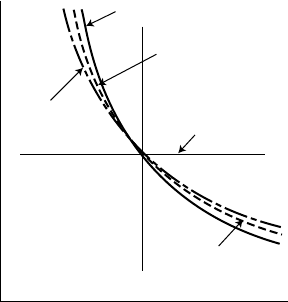
77 Basic fluid mechanics

well above their liquefication temperature will

approximate to it and so they can be considered

as a perfect gas.

5.1.3 Changes of state

When a perfect gas changes state its behaviour

approximates to:

pv

n

= constant

where n is known as the polytropic exponent.

Figure 5.1 shows the four main changes of

state relevant to aeronautics: isothermal,

adiabatic: polytropic and isobaric.

Specific volume,

v

Isobaric

n

= ∞

n

= κ

n

= 1

n

= 0

1<

n

<κ

Polytropic

Adiabatic

Isothermal

0

Pressure,

p

Fig. 5.1 Changes of state of a perfect gas

5.1.4 Compressibility

The extent to which a fluid can be compressed in

volume is expressed using the compressibility

coefficient



.

=

∆v/v

=

∆p

1



K

where ∆v = change in volume

v = initial volume

∆p = change in pressure

K = bulk modulus







 

78 Aeronautical Engineer’s Data Book

Also:

K =



∆p



∆



= 

dp



d



and

a =





=



d

K



p





d



where a = the velocity of propagation of a

pressure wave in the fluid

5.1.5 Fluid statics

Fluid statics is the study of fluids which are at rest

(i.e. not flowing) relative to the vessel containing

it. Pressure has four important characteristics:

• Pressure applied to a fluid in a closed vessel

(such as a hydraulic ram) is transmitted to

all parts of the closed vessel at the same

value (Pascal’s law).

• The magnitude of pressure force acting at

any point in a static fluid is the same,

irrespective of direction.

• Pressure force always acts perpendicular to

the boundary containing it.

• The pressure ‘inside’ a liquid increases in

proportion to its depth.

Other important static pressure equations are:

• Absolute pressure = gauge pressure +

atmospheric pressure.

• Pressure (p) at depth (h) in a liquid is given

by p =



gh.

• A general equation for a fluid at rest is

pdA – p +

dp



dz

dA –



gdAdz = 0

This relates to an infinitesimal vertical

cylinder of fluid.

5.2 Flow equations

Flow of a fluid may be one dimensional (1D),

two dimensional (2D) or three dimensional

79 Basic fluid mechanics

The stream tube for conservation of mass

1

2

v

1

v

2

p

1

p

2

A

1

A

2

s

z

s

α

δ

s

δ

s

dp

ds

p

The stream tube and element for the momentum equation

W

The forces on the element

F

pA

δ

s

W

α

(p+

d

p

d

s

(p+

d

p

δ

s

) (

A

+δ

A

)

d

s

δ

s

)

2

Control volume for the energy equation

s

1

2

z

1

v

2

p

2

T

2

p

2

v

1

p

1

T

1

p

1

z

2

q

α

Fig. 5.2 Stream tube/fluid elements: 1-D flow

(3D) depending on the way that the flow is

constrained.

5.2.1 1D Flow

1-D flow has a single direction co-ordinate x and

a velocity in that direction of u. Flow in a pipe

or tube is generally considered one dimensional.

80

Table 5.2 Fluid principles

Law Basis Resulting equations

Conservation of mass Matter (in a stream tube or anywhere else) cannot be

created or destroyed.

Conservation of momentum The rate of change of momentum in a given direction =

algebraic sum of the forces acting in that direction

(Newton’s second law of motion).

Conservation of energy Energy, heat and work are convertible into each other

and are in balance in a steadily operating system.

Equation of state Perfect gas state:

p/



T = r and the first law of

thermodynamics



vA = constant

dp



+

1



2

v

2

+ gz = constant∫





p

This is Bernoulli’s equation

2

v

c T +



= constant for an adiabatic (no heat

p

2

transferred) flow system

p = k



k = constant

 = ratio of specific heats c

p

/c

v

81 Basic fluid mechanics

The equations for 1D flow are derived by

considering flow along a straight stream tube

(see Figure 5.2). Table 5.2 shows the principles,

and their resulting equations.

5.2.2 2D Flow

2D flow (as in the space between two parallel

flat plates) is that in which all velocities are

parallel to a given plane. Either rectangular (x,y)

or polar (r,



) co-ordinates may be used to

describe the characteristics of 2D flow. Table 5.3

and Figure 5.3 show the fundamental equations.

Rectangular co-ordinates

v

u

y

x

u

+

∂

u

∂

x

δ

x

2

v

–

∂

v

∂

y

δ

y

δ

x

δ

y

2

u

–

∂

u

∂

x

δ

x

2

v

+

∂

v

∂

y

δ

y

2

P

Unit thickness

Polar co-ordinates

P(

r

,θ )

q

n

+

∂

q

n

q

n

∂

r

δ

r

δ

r

2

q

n

–

∂

q

n

∂

r

δ

r

2

∂

q

t

q

t

δθ

2

q

t

+

∂

q

t

∂θ

δθ

2

(

r

– )δθ

δ

r

2

(

r

+ )δθ

δ

r

2

q

t

–

∂θ

Fig. 5.3 The continuity equation basis in 2-D

 

82

Table 5.3 2D flow: fundamental equations

Basis The equation Explanation

Laplace’s equation

+ = 0 =

∂

2

∂

2

+

22





∂y





∂x

A flow described by a unique velocity

potential is irrotational.

∂

2

∂

2

2 2



or

2



= 

2



= 0, where

∂

2

∂

2





∂y





∂x



2

= +

22



∂y



∂x

Equation of motion in 2D

X –

∂p



∂x

The principle of force = mass  acceleration

(Newton’s law of motion) applies to fluids

and fluid particles.

∂u



∂t

+ u

∂u



∂x

+ v

∂u



∂y

=

1





∂v



∂t

+ u

∂v



∂x

+ v

∂v



∂t

=

1





Y –

∂p



∂y













83

Equation of continuity in 2D

(incompressible flow)

If fluid velocity increases in the x direction,

= 0 or, in polar

∂u



∂x

it must decrease in the y direction (see

+

Figure 5.3).

+

1



r

∂q

t

= 0

∂



q

n



r

+

∂v



∂y

∂q

n



∂r

Equation of vorticity A rotating or spinning element of fluid can

=



or, in polar:

be investigated by assuming it is a solid (see

∂v



∂x

–

Figure 5.4).

∂q

t

+



∂r

–

∂



∂q

n



1



=

r

Stream function



(incompressible flow)

Velocity at a point is given by:



is the stream function. Lines of constant



∂ ∂

∂x





∂y

give the flow pattern of a fluid stream (see

Figure 5.5).

u = v =

∂u



∂y

q

t



r

Velocity potential



(irrotational 2D flow)

Velocity at a point is given by:



is defined as:

∂ ∂

∂

y





∂x

=

 q cos



ds (see Figure 5.6).

u = v =

op

84 Aeronautical Engineer’s Data Book

∆

m

v

x

y

u

P(

x,y

)

0

Q(

x

+δ

x,y

+δ

y

)

u

+

∂

u

∂

x

δ

x

+

∂

u

∂

y

δ

y

v

+

∂

v

∂

x

δ

x

+

∂

v

∂

y

δ

y

Fig. 5.4 The vorticity equation basis in 2-D

y

x

u

0

ψ

ψ +

d

ψ

dQ

dy

B

A

dx

v

Fig. 5.5 Flow rate (q) and stream function (



) relationship

δ

s

β

q

sin β

q

cos β

q

Fig. 5.6 Velocity potential basis



  



  



2

85 Basic fluid mechanics

5.2.3 The Navier-Stokes equations

The Navier-Stokes equations are written as:

+u +v =



X– +µ



∂

2

u



∂x

2

+

u



∂y

∂

2

∂u



∂t

∂u



∂x

∂u



∂y

∂p



∂x

∂v



∂t

∂v



∂x

∂v



∂y

∂p



∂y

+µ



2

∂ v



∂x

+

2

∂ v



∂y

=



Y–+u +v

Inertia Body Pressure Viscous

term force term term

term

Source

y

O

ψ = constant, i.e. streamlines

radiating from the origin O.

φ = constant,

i.e. equipotential

lines centred at

the origin O.

x

If

q

>O this is a source of strength |

q

|

If

q

<O this is a sink of strength |

q

|

Flow due to a combination

ψ = constant

O

BA

y

x

φ = constant

of source and sink

Fig. 5.7 Sources, sinks and combination

86 Aeronautical Engineer’s Data Book

5.2.4 Sources and sinks

A source is an arrangement where a volume of

fluid (+q) flows out evenly from an origin

toward the periphery of an (imaginary) circle

around it. If q is negative, such a point is termed

a sink (see Figure 5.7). If a source and sink of

equal strength have their extremities infinitesi-

mally close to each other, whilst increasing the

strength, this is termed a doublet.

5.3 Flow regimes

5.3.1 General descriptions

Flow regimes can be generally described as

follows (see Figure 5.8):

Steady

Flow parameters at any point do

flow

not vary with time (even though

they may differ between points)

Unsteady

Flow parameters at any point vary

flow

with time

Laminar

Flow which is generally considered

flow

smooth, i.e. not broken up by eddies

Turbulent

Non-smooth flow in which any

flow

small disturbance is magnified,

causing eddies and turbulence

Transition

The condition lying between

flow

laminar and turbulent flow regimes

5.3.2 Reynolds number

Reynolds number is a dimensionless quantity

which determines the nature of flow of fluid

over a surface.

Inertia forces

Reynolds number (Re) =



Viscous forces



VD VD

=



=



µ



where



= density

µ = dynamic viscosity



= kinematic viscosity

V = velocity

D = effective diameter

Low Reynolds numbers (below about 2000)

result in laminar flow. High Reynolds numbers

(above about 2300) result in turbulent flow.

Basic fluid mechanics 87

‘Wake’ eddies move

slower than the rest

of the fluid

Steady flow

Unsteady flow

Boundary layer

Velocity distributions in laminar and turbulent flows

The flow is not steady

relative to any axes

Wake

Area of laminar flow

Area of turbulent flow

Boundary layer of

thickness (δ)

Turbulent flow

Laminar flow

v

u

max

u

The flow is steady, relative

to the axes of the body

Fig. 5.8 Flow regimes

88 Aeronautical Engineer’s Data Book

Values of Re for 2000 < Re < 2300 are gener-

ally considered to result in transition flow.

Exact flow regimes are difficult to predict in

this region.

5.4 Boundary layers

5.4.1 Definitions

The boundary layer is the region near a surface

or wall where the movement of the fluid flow

is governed by frictional resistance.

The main flow

is the region outside the

boundary layer which is not influenced by

frictional resistance and can be assumed to be

‘ideal’ fluid flow.

Boundary layer thickness: it is convention

to assume that the edge of the boundary layer

lies at a point in the flow which has a velocity

equal to 99% of the local mainstream

velocity.

5.4.2 Some boundary layer equations

Figure 5.9 shows boundary layer velocity

profiles for dimensional and non-dimensional

cases. The non-dimensional case is used to

allow comparison between boundary layer

profiles of different thickness.

Dimensional case Non-dimensional case

y

u

δ

Edge

of BL

0.99

U

∼

U

1

∼

∂

u

∂

y



y

=o

y

= y

y

u

Edge

of BL

u

= 1.0

u

= 1.0

δ

u

=

u

U

1

Fig. 5.9 boundary layer velocity profiles























89 Basic fluid mechanics

where:

µ = velocity parallel to the surface

y = perpendicular distance from the surface

= boundary layer thickness

U

1

= mainstream velocity

u = velocity parameters u/U

1

(non-dimensional)

y = distance parameter

y/



(non-dimensional)





∂y

Boundary layer equations of turbulent flow:





∂x

∂u ∂

u ∂p ∂





∂y





∂x

u + += –



= µ

∂u





∂y

–





u



v



'



'





∂y

∂p

= 0







∂y





∂x

∂u ∂

= 0+

5.5 Isentropic flow

For flow in a smooth pipe with no abrupt

changes of section:

d du



u

dA



A

continuity equation = 0+ +

equation of momentum

conservation

–dpA = (A



u)du

k



dp



d



p = cisentropic relationship

sonic velocity a

2

=

These lead to an equation being derived on the

basis of mass continuity:

dp





du



u

i.e.

or

= – M

2





d



d

M

2

=

du



u

 























 









90 Aeronautical Engineer’s Data Book

Table 5.4 Isentropic flows

Pipe flows

–dp du



u

= M

2

Convergent

Flow velocity u =

nozzle flows

k



2



–

ρ

0

Flow rate m =



uA





1



k

1

0



p



1 –

–1



k



p

ρ

k

0

Convergent-

2

k + 1

k– 1

p

0



p



1/k

divergent

nozzle flow

Area ratio

A



A*

=

k + 1

k –1

(1–





p

0



p





k)

k

1 –

Table 5.4 shows equations relating to conver-

gent and convergent-divergent nozzle flow.

5.6 Compressible 1D flow

Basic equations for 1D compressible flow are

Euler’s equation of motion in the steady state

along a streamline:

dp



ds

1





d



ds

1



2

u

2

= 0+

or

∫

dp





1



2

= constant+ u

so:

k

RT +

k – 1

1



2

u

2

= constant

T

0



T

p

0



p

=



k/(k – 1)

= 1 +

k – 1



k/(k – 1)

M

2

where T

0

= total temperature.

5.7 Normal shock waves

5.7.1 1D flow

A shock wave is a pressure front which travels

at speed through a gas. Shock waves cause an

increase in pressure, temperature, density and

entropy and a decrease in normal velocity.

Equations of state and equations of conser-

vation applied to a unit area of shock wave give

(see Figure 5.10):

State p

1

/



1

T

1

= p

2

/



2

T

2

Mass flow m =



1

u

1

=



2

u

2

Basic fluid mechanics 91

uu

1

p

1

p

2

Shock wave travels into area of stationary gas



Fig. 5.10(a) 1-D shock waves

uu

1

p

1

p

2

Shock wave becomes a stationary discontinuity



Fig. 5.10(b) Aircraft shock waves

92 Aeronautical Engineer’s Data Book

2

Momentum p

1

+ p

1

u

1

2

= p

2

+



2

u

2

2 2

u

1

u

2

Energy c T

1

+



= c

p

T

2

+



= c

p

T

0p

2 2

Pressure and density relationships across the

shock are given by the Rankine-Hugoniot

equations:



+ 1



2



– 1

p



–1



1

2



=



p



+ 1



2

1



–





–1



1

(



+ 1)p



2

+ 1



2

(



–1)p

1



=





1



+ 1 p

2



+





–1 p

1

Static pressure ratio across the shock is given

by:

p

1

2



M

2

– (



– 1)



=



p

2



+ 1

Temperature ratio across the shock is given by:

T

2

p

2



2



=



T

1

p

1

/



1

T

2



M

2

1

– (



+ 1) 2 + (



– 1)M

2

1



=



T

1





+ 1



(



+ 1)M

2



1

Velocity ratio across the shock is given by:

From continuity: u

2

/u

1

=



1

/



2

u

2

2 + (



– 1)M

2

so:



=



1

u

1

(



+ 1)M

2

1

In axisymmetric flow the variables are indepen-

dent of



so the continuity equation can be

expressed as:

1 ∂

(R

2

q

R

) 1 ∂(sin



q



)



+





= 0

R

2

∂R R sin



∂



Similarly in terms of stream function



:







93 Basic fluid mechanics

1 ∂



q

R

=



R

2

sin



∂



1 ∂



q



=



R sin



∂R

Additional shock wave data is given in Appen-

dix 5. Figure 5.10(b) shows the practical effect

of shock waves as they form around a super-

sonic aircraft.

5.7.2 The pitot tube equation

An important criterion is the Rayleigh super-

sonic pitot tube equation (see Figure 5.11).

M



 



/(



– 1)

2

1



+ 1

p

02

2

Pressure ratio:



=

p

1

2

M

1



1

p

1

u

1

p

2

p

02

M

2

Fig. 5.11 Pitot tube relations

2



M

2

1

– (



– 1)



+ 1

5.8 Axisymmetric flows

Axisymmetric potential flows occur when

bodies such as cones and spheres are aligned



94 Aeronautical Engineer’s Data Book

y

x

z

R

r

q

R

q

θ

q

ϕ

θ

ϕ





∂



Fig. 5.12 Spherical co-ordinates for axisymmetric flows





∂R

into a fluid flow. Figure 5.12 shows the layout

of spherical co-ordinates used to analyse these

types of flow.

Relationships between the velocity compo-

nents and potential are given by:

∂ ∂

R sin



1





∂



1



r

∂

q

R

=

q



=

q



=

5.9 Drag coefficients

Figures 5.13(a) and (b) show drag types and

‘rule of thumb’ coefficient values.

U

Shape Pressure drag Friction drag

D

P

(%) D

f

(%)

0 100

≈ 10 ≈ 90

≈ 90 ≈ 10

100 0

Fig. 5.13(a) Relationship between pressure and fraction

drag: ‘rule of thumb’

95 Basic fluid mechanics

d

l

d



l

U

Cylinder (flow direction)

Shape Dimensional

ratio

Datum

area, A

Approximate

drag

coefficient, C

D

Cylinder (right angles to flow)

Hemisphere (bottomless)

Cone

d

I

I/d

= 1 0.91

2 0.85

4 0.87

7 0.99

I/d

= 1 0.63

2 0.68

5 0.74

10 0.82

40 0.98

∞ 1.20

I 0.34

II 1.33

a

= 60˚ 0.51

a

= 30˚ 0.34

1.2

π

–

d

2

4

π

–

d

2

4

dl

π

–

d

2

4

π

–

d

2

4

Bluff bodies

Rough Sphere (

Re

= 10

6

) 0.40

Smooth Sphere (

Re

= 10

6

) 0.10

Hollow semi-sphere opposite stream 1.42

Hollow semi-sphere facing stream 0.38

Hollow semi-cylinder opposite stream 1.20

Hollow semi-cylinder facing stream 2.30

Squared flat plate at 90° 1.17

Long flat plate at 90° 1.98

Open wheel, rotating,

h

/

D

= 0.28 0.58

Streamlined bodies

Laminar flat plate (

Re

= 10

6

) 0.001

Re

= 10

6

) 0.005

0.006

0.025

0.05

0.16

0.005

0.09

n.a.

Aircraft -general

0.012

M

= 2.5 0.016

Airship 0.020–0.025

Helicopter download 0.4–1.2

II

Turbulent flat plate (

Airfoil section, minimum

Airfoil section, at stall

2-element airfoil

4-element airfoil

Subsonic aircraft wing, minimum

Subsonic aircraft wing, at stall

Subsonic aircraft wing, minimum

Subsonic aircraft wing, at stall

Aircraft wing (supersonic)

Subsonic transport aircraft

Supersonic fighter,

Fig. 5.13(b) Drag coefficients for standard shapes

Section 6

Basic aerodynamics

6.1 General airfoil theory

When an airfoil is located in an airstream, the

flow divides at the leading edge, the stagna-

tion point. The camber of the airfoil section

means that the air passing over the top

surface has further to travel to reach the trail-

ing edge than that travelling along the lower

surface. In accordance with Bernoulli’s

equation the higher velocity along the upper

airfoil surface results in a lower pressure,

producing a lift force. The net result of the

velocity differences produces an effect equiv-

alent to that of a parallel air stream and a

rotational velocity (‘vortex’) see Figures 6.1

and 6.2.

For the case of a theoretical finite airfoil

section, the pressure on the upper and lower

surface tries to equalize by flowing round the

tips. This rotation persists downstream of the

wing resulting in a long U-shaped vortex (see

Figure 6.1). The generation of these vortices

needs the input of a continuous supply of

energy; the net result being to increase the drag

of the wing, i.e. by the addition of so-called

induced drag

.

6.2 Airfoil coefficients

Lift, drag and moment (L, D, M) acting on an

aircraft wing are expressed by the equations:



U

2

Lift (L) per unit width = C

L

l

2



2

97 Basic aerodynamics

An effective rotational

velocity (vortex)

superimposed on the

parallel airstream

+

–

(

a)

Pressures equalize by flows

(

b)

around the tip

– – – – – – – –

+ + + + + + + +

Tip

Midspan

Tip

Core of vortex

(

c)

Finite airfoil

‘Horse-shoe’ vortex

persists downstream

Fig. 6.1 Flows around a finite 3-D airfoil

Camber line

edge

Chord

Camber

Thickness

Leading

edge

l

L

D

a

U

General airfoil section

Trailing

Profile of an asymmetrical airfoil section

Centre line

Chord line

x

t

c

Fig. 6.2 Airfoil sections: general layout

98 Aeronautical Engineer’s Data Book



U

2

Drag (D) per unit width = C

D

l

2



2

Moment (M) about LE or



U

2

1/4 chord = C

M

l

2



2

per unit width.

C

L

, C

D

and C

M

are the lift, drag and moment

coefficients, respectively. Figure 6.3 shows

typical values plotted against the angle of

attack, or incidence, (



). The value of C

D

is

small so a value of 10 C

D

is often used for the

characteristic curve. C

L

rises towards stall point

and then falls off dramatically, as the wing

enters the stalled condition. C

D

rises gradually,

increasing dramatically after the stall point.

Other general relationships are:

• As a rule of thumb, a Reynolds number of

Re  10

6

is considered a general flight

condition.

• Maximum C

L

increases steadily for

Reynolds numbers between 10

5

and 10

7

.

• C

D

decreases rapidly up to Reynolds

numbers of about 10

6

, beyond which the

rate of change reduces.

• Thickness and camber both affect the

maximum C

L

that can be achieved. As a

general rule, C

L

increases with thickness

and then reduces again as the airfoil

becomes even thicker. C

L

generally

increases as camber increases. The

minimum C

D

achievable increases fairly

steadily with section thickness.

6.3 Pressure distributions

The pressure distribution across an airfoil

section varies with the angle of attack (



).

Figure 6.4 shows the effect as



increases, and

the notation used. The pressure coefficient C

p

reduces towards the trailing edge.

99 Basic aerodynamics

Characteristics for an asymmetrical ‘infinite-span 2D airfoil’

75

50

25

0

–25

1.5

1.0

0.5

0

–0.5

–5˚

20˚15˚

10

C

D

10˚5˚

α

L/D

C

L

C

L

and 10

C

D

C

L

= 0 at the no-lift angle (–α)

Stall

point

Characteristic curves of a practical wing

2.0 0.20

1.6 0.16

C

L

C

D

C

M

1/4

1.2 0.12

0.8 0.08

0.4 0.04

C

L

C

M

1/4

C

D

0 0

–

0.4 –0.04

–

0.08

–0.12

–8˚ –4˚ 0˚ 4˚ 8˚ 12˚ 16˚ 20˚

α

Fig. 6.3 Airfoil coefficients

100 Aeronautical Engineer’s Data Book

Arrow length represents the magnitude of pressure coefficient

C

p

P

∞

= upstream

pressure

S

Stagnation point (S)

moves backwards on

the airfoil

lower surface

(

p

–

p

∞

)

α  5˚

S

Pressure coefficient

C

=

p

1



V

2

α  12˚

2

Fig. 6.4 Airfoil pressure coefficient (Cp)

6.4 Aerodynamic centre

The aerodynamic centre (AC) is defined as the

point in the section about which the pitching

moment coefficient (C

M

) is constant, i.e. does

not vary with lift coefficient (C

L

). Its theoreti-

cal positions are indicated in Table 6.1.

Table 6.1 Position of aerodynamic centre

Condition Theoretical positon of the AC



< 10° At approx. 1/4 chord

somewhere near the chord line.

Section with high At 50% chord.

aspect ratio

Flat or curved plate: At approx. 1/4 chord.

inviscid, incompressible

flow



101 Basic aerodynamics

Using common approximations, the following

equations can be derived:

d

(C

Ma

)

dC

L

= –

x

AC



c

9



c

where C

Ma

= pitching moment coefficient at

distance a back from LE

x

AC

= position of AC back from LE.

c = chord length.

6.5 Centre of pressure

The centre of pressure (CP) is defined as the

point in the section about which there is no

pitching moment, i.e. the aerodynamic forces

on the entire section can be represented by lift

and drag forces acting at this point. The CP

does not have to lie within the airfoil profile

and can change location, depending on the

magnitude of the lift coefficient C

L

. The CP is

conventionally shown at distance k

CP

back from

the section leading edge (see Figure 6.5). Using

Lift and drag only cut at the CP

C

x

AC

M

AC

M

LE

Lift

Drag

Aerodynamic centre

Lift

k

CP

M

Drag

Centre of pressure (CP)

Fig. 6.5 Aerodynamic centre and centre of pressure

102 Aeronautical Engineer’s Data Book

the principle of moments the following expres-

sion can be derived for k

CP

:

x

AC

C

M

AC

k

CP

=



–



c C

L

cos



+ C

D

sin



Assuming that cos



1 and C

D

sin



 0 gives:

x

AC

C

M

AC

k

CP





–



c C

L

6.6 Supersonic conditions

As an aircraft is accelerated to approach super-

sonic speed the equations of motion which

describe the flow change in character. In order

to predict the behaviour of airfoil sections in

upper subsonic and supersonic regions,

compressible flow equations are required.

6.6.1 Basic definitions

M Mach number

M

∞

Free stream Mach number

M

c

Critical Mach number, i.e. the value of

which results in flow of M

∞

= 1 at some

location on the airfoil surface.

Figure 6.6 shows approximate forms of the

pressure distribution on a two-dimensional airfoil

around the critical region. Owing to the complex

non-linear form of the equations of motion which

describe high speed flow, two popular simplifica-

tions are used: the small perturbation approxima-

tion and the so-called exact approximation.

6.6.2 Supersonic effects on drag

In the supersonic region, induced drag (due to

lift) increases in relation to the parameter



M

2

– 1



function of the plan form geometry of

the wing.

6.6.3 Supersonic effects on aerodynamic centre

Figure 6.7 shows the location of wing aerody-

namic centre for several values of tip chord/root

chord ratio (



). These are empirically based

results which can be used as a ‘rule of thumb’.

103

0

Basic aerodynamics

M1 (local)

M

∞

> M

crit

M

∞

> M

crit

–1.2

–0.8

–0.4

–C –C

p p

0.4

0.8

1.2

0 0.2 0.4 0.6 0.8 1.0

x/c

M

∞

>> M

crit

Supersonic

regions

–

0.8

–0.4

–1.2

–C

p

0

0.4

0.8

1.2

0 0.2 0.4 0.6 0.8 1.0

x/c

Fig. 6.6 Variation of pressure deterioration (2-D airfoil)

6.7 Wing loading: semi-ellipse assumption

The simplest general loading condition assump-

tion for symmetric flight is that of the semi-

ellipse. The equivalent equations for lift,

downwash and induced drag become:

For lift:

VK

0

πs

L =





2

1

replacing L by C

L

/

2



V

2

S gives:

C

L

VS

K

0

=



πs

104 Aeronautical Engineer’s Data Book

2.0

1.8

1.6

1.4

X

a.c.

1.2

C

r

1.0

0.8

0.6

0.4

0.2

1.4

1.2

1.0

X

a.c.

0.8

C

r

0.6

0.4

0.2

0

1.2

1.0

X

a.c.

0.8

C

r

0.6

0.4

0.2

0

1 0 1 0

tanΛ

LE

β β tanΛ

LE

λ =

C

t

/

C

R

= 1.0

C

t

/

C

R

= 0.5

C

t

/

C

R

= 0.25

AR tanΛ

LE

AR tanΛ

LE

6

5

4

3

2

1

6

5

4

3

2

1

AR tanΛ

LE

6

5

4

3

2

1

Subsonic Supersonic

Unswept T.E.

Sonic T.E.

Taper ratio

β tanΛ

LE

tanΛ

LE

β

Fig. 6.7 Wing aerodynamic centre location: subsonic/

supersonic flight. Originally published in The AIAA

Aerospace Engineers Design Guide, 4th Edition. Copyright

Astronautics Inc. Reprinted with permission.



105 Basic aerodynamics

For downwash velocity (w):

w =

K

0



4S

, i.e. it is constant along the span.

For induced drag (vortex):

C

L

2

πAR

D

=

V

where aspect ratio (AR) =

2

span 4s

2

=

area



S

Hence, C

D

V

falls (theoretically) to zero as aspect

ratio increases. At zero lift in symmetric flight,

C

D

= 0.

V

Section 7

Principles of flight dynamics

7.1 Flight dynamics – conceptual breakdown

Flight dynamics is a multi-disciplinary subject

consisting of a framework of fundamental

mathematical and physical relationships.

Figure 7.1 shows a conceptual breakdown of

the subject relationships. A central tenet of the

framework are the equations of motion, which

provide a mathematical description of the

physical response of an aircraft to its controls.

7.2 Axes notation

Motions can only be properly described in

relation to a chosen system of axes. Two of the

most common systems are earth axes and

aircraft body axes.

The equations of motion

and handling

properties

Aerodynamic

characteristics

Common

aerodynamic

parameters

Stability and

control

derivatives

Stability and

control

parameters

Aircraft flying

of the airframe

Fig. 7.1 Flight dynamics – the conceptual breakdown

107 Principles of flight dynamics

Conventional earth axes are used as a reference frame for

‘short-term’ aircraft motion.

S

N

y

0

z

0

o

0

x

0

y

E

z

E

x

E

o

E

• The horizontal plane

o

E

,

x

E

,

y

E

, lies parallel to the plane

o

0

,

x

0

,

y

0

, on

the earth’s surface.

• The axis

o

E

,

z

E

, points vertically downwards.

Fig. 7.2 Conventional earth axes

7.2.1 Earth axes

Aircraft motion is measured with reference to a

fixed earth framework (see Figure 7.2). The

system assumes that the earth is flat, an assump-

tion which is adequate for short distance flights.

7.2.2 Aircraft body axes

Aircraft motion is measured with reference to

an orthogonal axes system (Ox

b

, y

b

, z

b

) fixed on

the aircraft, i.e. the axes move as the aircraft

moves (see Figure 7.3).

7.2.3 Wind or ‘stability’ axes

This is similar to section 7.2.2 in that the axes

system is fixed in the aircraft, but with the Ox-

axis orientated parallel to the velocity vector V

0

(see Figure 7.3).

7.2.4 Motion variables

The important motion and ‘perturbation’

variables are force, moment, linear velocity,

angular velocity and attitude. Figure 7.4 and

Table 7.1 show the common notation used.

7.2.5 Axes transformation

It is possible to connect between axes refer-

ences: e.g. if Ox

0

, y

0

, z

0

are wind axes and

components in body axes and



,



,



are the

angles with respect to each other in roll, pitch

and yaw, it can be shown that for linear quanti-

ties in matrix format:



= D



Ox

0

Oy

0

Oz

0

Ox

3

Oy

3

Oz

3

108 Aeronautical Engineer’s Data Book

x

b

x

w

z

b

z

w

y

b,

.y

w

V

0

Conventional body axis system.

O

x

b

is parallel to the ‘fuselage horizontal’ datum

O

z

b

is ‘vertically downwards’

O

Conventional wind (or‘stability’) axis

system: O

x

w

is parallel to the velocity vector

V

o

Roll

L,p,

φ

Pitch

M,q,

θ

Yaw

N,r,

ψ

X,U

e

,U,u

Z,W

e

,W,w

Y

,V

e

,V,v

Fig. 7.3 Aircraft body axes

Fig. 7.4 Motion variables: common notation











 

 

109 Principles of flight dynamics

Table 7.1 Motion and perturbation notation

Perturbations

Aircraft axis Ox

Force X

Moment L

Linear velocity U

Angular velocity p

Attitude



Oy Oz

Y Z

M N

V W

q r

Motions

X Axial ‘drag’ force

Y Side force

Z Normal ‘lift’ force

L Rolling moment

M Pitching moment

N Yawing moment

p Roll rate

q Pitch rate

r Yaw rate

U Axial velocity

V Lateral velocity

W Normal velocity

Where the direction cosine matrix D is given

by:

cos



cos



cos



cos



– sin



sin



sin



cos



sin



sin



sin



sin



cos



D =



– cos



sin



+ cos



sin



cos



sin



cos



cos



sin



cos



cos



cos



+ sin



sin



– sin



cos



Angular velocity transformations can be

expressed as:

p 1

0

–sin





q =



0 cos



sin



cos







r 0 –sin



cos



cos





where p, q, r are angular body rates:

Roll rate p =



–



sin





,



,



where



Pitch rate q =



cos



are attitude

+



sin



cos



rates with



respect to

Yaw rate r =



cos



cos



datum axes

–



sin







110 Aeronautical Engineer’s Data Book

Inverting gives:



1 sin



tan



cos



tan



p



=



0 cos



–sin



q

  



0 sin



sec



cos



sec



r

7.3 The generalized force equations

The equations of motions for a rigid aircraft are

derived from Newton’s second law (F = ma)

expressed for six degrees of freedom.

7.3.1 Inertial acceleration components

To apply F = ma, it is first necessary to define

acceleration components with respect to earth

(‘inertial’) axes. The equations are:

1

a

x

= U – rV + qW – x(q

2

+ r

2

) + y(pq – r)

+ z(pr + q)

1

a

y

= V – pW + rU + x(pq + r) – y(p

2

+ r

2

)

+ x(qr – p)

1

a

z

= W – qU + pV = x(pr – q) + y(qr + p)

– z(p

2

+ q

2

)

1 1

where: a

1

x

, a

y

, a are vertical acceleration

z

components of a point p(x, y, z) in the rigid

aircraft.

U, V, W are components of velocity along the

axes Ox, Oy, Oz.

p, q, r are components of angular velocity.

7.3.2 Generalized force equations

The generalized force equations of a rigid body

(describing the motion of its centre of gravity)

are:

m(U – rV + qW) = X where m is

m(V – pW + rU) = Y the total mass

m(W – qU + pV) = Z of the body

7.4 The generalized moment equations

A consideration of moments of forces acting at

a point p(x, y, z) in a rigid body can be

expressed as follows:



111 Principles of flight dynamics

Moments of inertia

I

x

= ∑



m(y

2

+ z

2

) Moment of inertia about

Ox axis

I

I = ∑



m(x

2

+ z

2

) Moment of inertia about

Oy axis

z

= ∑



m(x

2

+ y

2

) Moment of inertia about

Oz axis

I

y

I

= ∑



m xy Product of inertia about

Ox and Oy axes

xz

= ∑



m xz Product of inertia about

Ox and Oz axes

I = ∑



m yz Product of inertia about

xy

yz

Oy and Oz axes

The simplified moment equations become

I

x

p



– (I

y

– I

z

) qr – I

xz

(pq + r



) = L

2

I

y

q



– (I

x

– I

z

) pr – I

xz

(p – r

2

) = M



I

z

r



– (I

x

– I

y

) pq – I

xz

(qr + p



) = N

7.5 Non-linear equations of motion

The generalized motion of an aircraft can be

expressed by the following set of non-linear

equations of motion:

m(U – rV + qW

) = X

a

+ X

g

+ X

c

+ X + X

dp

m(V – pW + rU) = Y

a

+ Y + Y

c

+ Y

p

+ Y

dg

m(W – qU + pV) = Z

a

+ Z

g

+ Z

c

+ Z + Z

dp

I

x

p



– (I

y

– I

x

) qr – I

xz

(pq + r



) = L

a

+ L

g

+

L

c

+ L

p

+ L

d



2

I

M

I

y

q



+ (I

x

– I

z

) pr + I

xz

(p – r

2

) = M

a

+ M

g

+

c

+ M

p

+ M

d

z

r



– (I

x

– I

y

) pq + I

xz

(qr – p



) = N

a

+ N +

g

N

c

+ N

p

+ N

d

7.6 The linearized equations of motion

In order to use them for practical analysis, the

equations of motions are expressed in their

linearized form by using the assumption that all

perturbations of an aircraft are small, and

about the ‘steady trim’ condition. Hence the

equations become:





112 Aeronautical Engineer’s Data Book

m(u + qW

e

) = X

a

+ X + X

c

+ X

p

m(v + pW

e

+ rU

e

) = Y

a

+ Y

g

+ Y

c

+ Y

g

p

m(w + qU

e

) = Z

a

+ Z

g

+ Z

c

+ Z

p

I

x

p – I

xz

r = L

a

+ L

g

+ L

c

+ L

p

I

y

q = M

a

+ M + M

c

+ M

pg

I

z

r – I

xz

p = N

a

+ N

g

+ N

c

+ N

p

A better analysis is obtained by substituting

appropriate expressions for aerodynamic,

gravitational, control and thrust terms. This

gives a set of six simultaneous linear differen-

tial equations which describe the transient

response of an aircraft to small disturbances

about its trim condition, i.e.:

mu – X

˚

u

u – X

˚

v – X

˚

w

w – X

˚

w

v w

–X

˚

p

p – (X

˚

– mW

e

)

q

– X

˚

r

r + mg



cos



=

X

˚



+ X

˚



+ X

˚



+ X

˚



q e

–Y

˚

u

u + mv – Y

˚

v – Y

˚

w

w – Y

˚

w – (Y

˚

p

+

mW

e

)p

v w

–Y

˚

q

q – (Y

˚

– mU

e

)r – mg



cos



e

– mg



sin



= Y

˚



+ Y

˚



= Y

˚



+ Y

˚



r

e

–Z

˚

u

u – Z

˚

v + (m – Z

˚

w) w – Z

˚

w

v w w

–Z

˚

p

p – (Z

˚

– mU

e

)

q

– Z

˚

r

r + mg



sin



=

Z

˚



+ Z

˚



= Z

˚



+ Z

˚



q e

–L

˚

u

u – L

˚

v – L

˚

w

w – L

˚

w

v w

+I

x

p – L

˚

p

p – L

˚

q

q – I

xz

r – L

˚

r = L

˚



+ L

˚



= L

˚



+ L

˚



r

˚ ˚

–M

u

u – M

˚

v

v – M

w

˚ ˚ ˚

–M

w

w – M

p

p – + I

y

q – M

q

q – M

˚

r = M

˚



˚ ˚

r

+ M



= M

˚



+ M



˚ ˚

–N

u

u – N

˚

v

v – N

˚

w

w – N

w

˚ ˚ ˚ ˚

I

xz

p – N

p

p – N

q

q + I

z

r – N

˚

r

r = N



+ N

˚ ˚



= N



+ N



113

Table 7.2 Stability terms

Term Meaning

Static stability The tendency of an aircraft to converge back to its equilibrium condition after a small disturbance from trim.

Lateral static stability The tendency of an aircraft to maintain its wings level in the roll direction.

Directional static stability The tendency of an aircraft to ‘weathercock’ into the wind to maintain directional equilibrium.

Dynamic stability The transient motion involved in recovering equilibrium after a small disturbance from trim.

Degree of stability A parameter expressed by reference to the magnitude of the slope of the C

m

–



, C

1

–



and C

n

–



characteristics.

Stability margin The amount of stability in excess of zero or neutral stability.

Stability reversal Change in sign of pitching moment coefficient (C

m

) at high values of lift coefficient (C

L

). The result is an

unstable pitch-up characteristic (see Figures 7.6 and 7.7).

‘Controls fixed’ stability Stability of an aircraft in the condition with its flying control surfaces held at a constant setting for the

prevailing trim condition.

‘Controls free’ stability Stability of an aircraft in the condition with its flying control surfaces (elevator) free to float at an angle

corresponding to the prevailing trim condition.

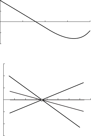
114 Aeronautical Engineer’s Data Book

7.7 Stability

Stability is about the nature of motion of an

aircraft after a disturbance. When limited by

the assumptions of the linearized equations of

motion it is restricted to the study of the motion

after a small disturbance about the trim condi-

tion. Under linear system assumptions, stability

is independent of the character of the disturb-

ing force. In practice, many aircraft display

distinctly non-linear characteristics. Some

useful definitions are given in Table 7.2, see

also Figures 7.5 and 7.6

Lift coefficient

C

L

Pitching moment coefficient

C

m

0.2

0.1

0.0

0 0 0.5 1.0 1.5 2.0

–0.1

–0.2

Fig. 7.5 Stability reversal at high lift coefficient

O

Nose

up

Nose

down

1

2

3

4

point

Incidence 



e

Pi

tc

hi

ng moment coe

ffi

c

i

ent

C

m

2 Stable

3 Neutral stability

4 Unstable

Trim

1 Very stable

Fig. 7.6 Degree of stability (static, longitudinal)

Section 8

Principles of propulsion

8.1 Propellers

A propeller or airscrew converts the torque of

an engine (piston engine or turboprop) into

thrust. Propeller blades have an airfoil section

which becomes more ‘circular’ towards the hub.

The torque of a rotating propeller imparts a

rotational motion to the air flowing through it.

Pressure is reduced in front of the blades and

increased behind them, creating a rotating

slipstream. Large masses of air pass through the

propeller, but the velocity rise is small compared

to that in turbojet and turbofan engines.

8.1.1 Blade element design theory

Basic design theory considers each section of

the propeller as a rotating airfoil. The flow over

the blade is assumed to be two dimensional (i.e.

no radial component). From Figure 8.1 the

following equations can be expressed:

Pitch angle



= tan

–1

(V

0

/πnd)

The propulsion efficiency of the blade element,

i.e. the blading efficiency, is defined by:

V

0

dF tan



L/D – tan





b

=



=



=



udQ tan(



+



) L/D + cot



u = velocity of blade element = 2πnr

where D = drag

L = lift

dF = thrust force acting on blade

element

dQ = corresponding torque force

r = radius

116 Aeronautical Engineer’s Data Book

Vector diagram for a blade element of a propeller

O'

A'

A

β

φ

b

w

α

B

V

o

Projection of

axis of rotation

c

O

u =

ωr = 2πrn

a

Aerodynamic forces acting on a blade element

Chord line

Projection of axis

of rotation

O'

α

O

90˚

dF

φ

γ

dR

dQ

A

e

c

b

d

dD

dL

–w

a

Fig. 8.1 Propeller blade elements

The value of



which makes



b

a maximum is

termed the optimum advance angle



opt

.

Maximum blade efficiency is given by:

2



– 1 2(L/D) – 1

(



b

)

max

=



=



2



+ 1 2(L/D) + 1

8.1.2 Performance characteristics

The pitch and angle



have different values at

different radii along a propeller blade. It is

common to refer to all parameters determining

the overall characteristics of a propeller to their

values at either 0.7r or 0.75r.

Lift coefficient C

L

is a linear function of the

angle of attack (



) up to the point where the

117 Principles of propulsion

Blading efficiency, η

s

1.00

0.80

0.60

0.40

0.20

0

10

20

30

8

6

4

3

L

= 2

D

0 10 20 30 40 50 60 70 80 90

Pitch angle, φ

Fig. 8.2 Propeller parameter relationship

blade stalls whilst drag coefficient C

D

is

quadratic function of



. Figure 8.2 shows broad

relationships between blading efficiency, pitch

angle and L/D ratio.

8.1.3 Propeller coefficients

It can be shown, neglecting the compressibility

of the air, that:

f(V

0

, n, d

p

,



, F) = 0

Using dimensional analysis, the following

coefficients are obtained for expressing the

performances of propellers having the same

geometry:

F =



n

2

d

4

p

C

F

Q =



n

2

d

5

p

C

Q

P =



n

3

d

5

C

p p

C

F

, C

Q

and C

P

are termed the thrust, torque,

and power coefficients. These are normally

expressed in USCS units, i.e.:

F

Thrust coefficient C

F

=





n

2

d

4

Q

Torque coefficient C

Q

=





n

2

d

5

P

Power coefficient C

P

=





n

3

d

4

118 Aeronautical Engineer’s Data Book

where d = propeller diameter (ft)

n = speed in revs per second

Q = torque (ft lb)

F = thrust (lbf)

r



R

P = power (ft

lb/s)



= air density (lb s

2

/ft

4

)

r



R

8.1.4 Activity factor

Activity factor (AF) is a measure of the power-

c



d

P

absorbing capabilities of a propeller, and

hence a measure of its ‘solidity’. It is defined

as:

16



3

d



AF =

100 000



r/R=1

r

h

/R

8.1.5 Propeller mechanical design

Propeller blades are subjected to:

• Tensile stress due to centrifugal forces.

• Steady bending stress due to thrust and

torque forces.

• Bending stress caused by vibration.

Vibration-induced stresses are the most serious

hence propellers are designed so that their first

order natural reasonant frequency lies above

expected operating speeds. To minimize the

chance of failures, blades are designed using

fatigue strength criteria. Steel blades are often

hollow whereas aluminium alloy ones are

normally solid.

8.2 The gas turbine engine: general

principles

Although there are many variants of gas

turbine-based aero engines, they operate using

similar principles. Air is compressed by an

axial flow or centrifugal compressor. The

highly compressed air then passes to a combus-

tion chamber where it is mixed with fuel and

ignited. The mixture of air and combustion

products expands into the turbine stage which

in turn provides the power through a coupling

shaft to drive the compressor. The expanding

119 Principles of propulsion

gases then pass out through the engine tailpipe,

providing thrust, or can be passed through a

further turbine stage to drive a propeller or

helicopter rotor. For aeronautical applications

the two most important criteria in engine

choice are thrust (or power) and specific fuel

consumption. Figure 8.3 shows an outline of

Turbojet

Optional afterburner (reheater) for military use

Power from gas

thrust only

Compressor Combustion

chamber

Turbofan (fan-jet)

Thrust reverser cowls

propeller

Shaft power

Output

(e.g. to drive helicopter rotor)

Bypass air merges

with gas thrust

Gas thrust

Fan

Extra tubine stage

Propeller thrust

Turboprop

Turbine-driven

Turboshaft

Fig. 8.3 Gas turbine engine types

120 Aeronautical Engineer’s Data Book

Engine efficiency (%)

100

90

Turboprop

80

70

T

urbofan

60

Turbojet

50

0.5

0.6 0.7 0.8 0.9

Mach No. (cruise)

Fig. 8.4 ‘Order of magnitude’ engine efficiencies

the main types and Figure 8.4 an indication of

engine efficiency at various flight speeds.

8.2.1 The simple turbojet

The simple turbojet derives all its thrust from

the exit velocity of the exhaust gas. It has no

separate propeller or ‘power’ turbine stage.

Performance parameters are outlined in Figure

8.5. Turbojets have poor fuel economy and high

exhaust noise. The fact that all the air passes

through the engine core (i.e. there is no bypass)

is responsible for the low propulsive efficiency,

except at very high aircraft speed. The

Concorde supersonic transport (SST) aircraft is

virtually the only commercial airliner that still

uses the turbojet. By making the convenient

assumption of neglecting Reynolds number,

the variables governing the performance of a

simple turbojet can be grouped as shown in

Table 8.1.

121 Principles of propulsion

0.3

0.2

0.1

1.6

1.2

0.8

0.4

Dimensionless specific thrust parameter

Overall efficiency η

0

λ

λ =

f

(

P

3

/

P

2

)

for α = 5

η

0

=

f

(

P

3

/

P

2

)

for α = 5

η

0

=

f

(α)

for

P

3

/

P

2

= 10

1 3 7 11 15

Compressor pressure ratio P

3

/P

2

2 4 6 8

Cycle temperature ratio α = T

4

/t

0

Fig. 8.5 Turbojet performance indicative design points

Table 8.1 Turbojet performance parameter groupings

Non-dimensional Uncorrected Corrected

group

Flight speed V

0

/



t

0



V

0







Rpm N/



T



N/







Air flow rate W

·

a

/



T/D

2

P



W

·

a

/





/





Thrust F/D

2

P F/



Fuel flow rate W

·

f

J∆H

c

/D

2

P



T



W

·

f

/ 









= T/T

std

= T/519 (T/288) = corrected temperature



= P/p

std

= P/14.7 (P/1.013  10

5

) = corrected pressure

·

W

f

= fuel flow

8.2.2 Turbofan

Most large airliners and high subsonic trans-

port aircraft are powered by turbofan

engines. Typical commercial engine thrust

ratings range from 7000 lb (31 kN) to

90 000 lb (400 kN+) suitable for large aircraft

such as the Boeing 747. The turbofan is

122 Aeronautical Engineer’s Data Book

characterized by an oversized fan compressor

stage at the front of the engine which

bypasses most of the air around the outside of

the engine where it rejoins the exhaust gases

at the back, increasing significantly the avail-

able thrust. A typical bypass ratio is 5–6 to 1.

Turbofans have better efficiency than simple

turbojets because it is more efficient to accel-

erate a large mass of air moderately through

the fan to develop thrust than to highly accel-

erate a smaller mass of air through the core

of the engine (i.e. to develop the same thrust).

Figure 8.3 shows the basic turbofan and

Figure 8.6 its two- and three-spool variants.

The two-spool arrangement is the most

common, with a single stage fan plus turbine

High pressure (hp) spool: The hp turbine (HPT)drives the high

pressure compressor (HPC)

Two spool (most common aero-engine configuration)

Core nozzle

Bypass nozzle

LPC

HPC

LPT

HPT

Fan

Three spool engine (Rolls-Royce RB211)

Fan

IPC HPC

HPT IPT

LPT

Low pressure spool: the lp turbine (LPT) drives the low

pressure compressor (LPC)

Third spool or

'free power'

drive to inlet fan

Fig. 8.6 Turbofan: 2- and 3-spool variants

123 Principles of propulsion

on the low pressure rotor and an axial

compressor plus turbine on the high pressure

rotor. Many turbines are fitted with thrust

reversing cowls that act to reverse the direc-

tion of the slipstream of the fan bypass air.

8.2.3 Turboprop

The turboprop configuration is typically used

for smaller aircraft. Data for commercial

models are shown in Table 8.2. The engine (see

Figure 8.3) uses a separate power turbine stage

to provide torque to a forward-mounted

propeller. The propeller thrust is augmented by

gas thrust from the exhaust. Although often

overshadowed by the turbofan, recent devel-

opments in propeller technology mean that

smaller airliners such as the SAAB 2000 (2 

4152 hp (3096 kW) turboprops) can compete

on speed and fuel cost with comparably sized

turbofan aircraft. The most common turboprop

configuration is a single shaft with centrifugal

compressor and integral gearbox. Commuter

airliners often use a two- or three-shaft ‘free

turbine’ layout.

8.2.4 Propfans

Propfans are a modern engine arrangement

specifically designed to achieve low fuel

consumption. They are sometimes referred to

as inducted fan engines. The most common

arrangement is a two-spool gas generator and

aft-located gearbox driving a ‘pusher’ fan.

Historically, low fuel prices have reduced the

drive to develop propfans as commercially

viable mainstream engines. Some Russian

aircraft such as the Anotov An-70 transport

have been designed with propfans.

8.2.5 Turboshafts

Turboshaft engines are used predominantly for

helicopters. A typical example such as the

Rolls-Royce Turbomeca RTM 32201 has a

three-stage axial compressor direct-coupled to a

two-stage compressor turbine, and a two-stage

Table 8.2 Aircraft engines – basic data

Company Allied CFE CFMI General Electric (GE) IAE (PW, RR, Pratt & Witney Rolls-Royce ZMKB

Signal MTU, JAE)

Engine LF507 CFE738 CFM 56 CF34 CF6 GE 90 V2522 V2533 PW4052 PW4056 PW4168 PW4084 TRENT TAY RB-211- D-436T1

type/Model 5C2 3A,3B 80E1A2 85B A5 A5 772 611 524H

Aircraft BA146-300 Falcon A340 Canadair A330 B777- MD90- A321- B767-200 B747-400 A330 B777 A330 F100.70 B747-400 Tu-334-1

Avro RJ 2000 RJ 200/300 10/30 200 &200ER 767-300ER Gulfst V B767-300 An 72,74

A319

In service date 1991 1992 1994 1996 1995 1993 1994 1986 1987 1993 1994 1995 1988 1989 1996

Thrust (lb) 7000 5918 31 200 9220 67 500 90 000 22 000 33 000 52 200 56 750 68 000 84 000 71 100 13 850 60 600 16 865

Flat rating (°C) 23 30 30 30 30 30 30 33.3 33.3 30 30 30 30 30 30

Bypass ratio 5.6 5.3 6.4 5 4.6 4.85 4.85 5.1 6.41 4.89 3.04 4.3 4.95

Pressure ratio 13.8 23 31.5 21 32.4 39.3 24.9 33.4 27.5 29.7 32 34.2 36.84 15.8 33 25.2

Mass flow (lb/s) 256 240 1065 1926 3037 738 848 1705 1705 1934 2550 1978 410 1605

SFC (lb/hr/lb) 0.406 0.369 0.32 0.35 0.33 0.34 0.37 0.351 0.359 0.43 0.563

Climb

Max thrust (lb) 7580 18 000 5550 6225 15 386 3400 12 726

Flat rating (°C) ISA+10 ISA+10 ISA+10 ISA+5 ISA+10

Cruise

Altitude (ft) 40 000 35 000 35 000 35 000 35 000 35 000 35 000 35 000 35 000 35 000 35 000 35 000 36 089

Mach number 0.8 0.8 0.83 0.8 0.8 0.8 0.8 0.8 0.83 0.82 0.8 0.85 0.75

Thrust (lb) 1310 5185 5725 11500 2550 11813 3307

Thrust lapse rate 0.2 0.174 0.162 0.184 0.195 0.196

Flat rating (°C) ISA+10 ISA+10 ISA+10 ISA+10

SFC (lb/hr/lb) 0.414 0.645 0.545 0.562 0.545 0.574 0.574 0.565 0.69 0.57 0.61

Dimensions

Length (m) 1.62 2.514 2.616 2.616 4.343 5.181 3.204 3.204 3.879 3.879 4.143 4.869 3.912 2.59 3.175

Fan diameter (m) 1.272 1.219 1.945 1.245 2.794 3.404 1.681 1.681 2.477 2.477 2.535 2.845 2.474 1.52 2.192 1.373

Basic eng. 1385 1325 5700 1670 10 726 16 644 5252 5230 9400 9400 14 350 13 700 10 550 2951 9670 3197

weight (lb)

Layout

Number of shafts 2 2 2 2 2 2 2 2 2 2 2 2 3 2 3 3

Compressor various 1+5LP 1+4LP 1F 1+4LP 1+3LP 1+4LP 1+4LP 1+4LP 1+4LP 1+5LP 1+6LP 1LP 8IP 1+3LP 1LP 7IP 1+1L 6I

+1CF 9HP +14cHP 14HP 10HP 10HP 10HP 11HP 11HP 11HP 11HP 6HP 12HP 6HP 7HP

Turbine 2HP 2HP 1HP 2HP 2HP 2HP 2HP 2HP 2HP 2HP 2HP 2HP 1HP 1IP 2HP 1HP 1IP 1HP 1IP

2LP 3LP 5LP 4LP 5LP 6LP 5LP 5LP 4LP 4LP 5LP 7LP 4LP 3LP 3LP 3LP

126 Aeronautical Engineer’s Data Book

power turbine. Drive is taken off the power

turbine shaft, through a gearbox, to drive the

main and tail rotor blades. Figure 8.3 shows the

principle.

8.2.6 Ramjet

This is the crudest form of jet engine. Instead

of using a compressor it uses ‘ram effect’

obtained from its forward velocity to accelerate

and pressurize the air before combustion.

Hence, the ramjet must be accelerated to speed

by another form of engine before it will start to

work. Ramjet-propelled missiles, for example,

are released from moving aircraft or acceler-

ated to speed by booster rockets. A supersonic

version is the scramjet which operates on liquid

hydrogen fuel.

8.2.7 PULSEJET

A pulsejet is a ramjet with an air inlet which is

provided with a set of shutters fixed to remain

in the closed position. After the pulsejet engine

is launched, ram air pressure forces the shutters

to open, and fuel is injected into the combus-

tion chamber and burned. As soon as the

pressure in the combustion chamber equals the

ram air pressure, the shutters close. The gases

produced by combustion are forced out of the

jet nozzle by the pressure that has built up

within the combustion chamber. When the

pressure in the combustion chamber falls off,

the shutters open again, admitting more air,

and the cycle repeats.

8.3 Engine data lists

Table 8.2 shows indicative design data for

commercially available aero engines from

various manufacturers.

8.4 Aero engine terminology

See Table 8.3.

127 Principles of propulsion

Table 8.3

Afterburner

A tailpipe structure attached to the back of military fighter

aircraft engine which provides up to 50% extra power for

short bursts of speed. Spray bars in the afterburner inject

large quantities of fuel into the engine’s exhaust stream.

Airflow

Mass (weight) of air moved through an engine per

second. Greater airflow gives greater thrust.

Auxiliary power Units (APUs)

A small (< 450 kW) gas turbine used to provide ground

support power.

Bleed air

Air taken from the compressor section of an engine for

cooling and other purposes.

Bypass Ratio (BPR)

The ratio of air ducted around the core of a turbofan

engine to the air that passes through the core. The air

that passes through the core is called the primary airflow.

The air that bypasses the core is called the secondary

airflow. Bypass ratio is the ratio between secondary and

primary airflow.

Combustion chamber

The section of the engine in which the air passing out of

the compressor is mixed with fuel.

Compressor

The sets of spinning blades that compress the engine air

stream before it enters the combustor. The air is forced

into a smaller and smaller area as it passes through the

compressor stages, thus raising the pressure ratio.

Compressor Pressure Ratio (CPR)

The ratio of the air pressure exiting the compressor

compared to that entering. It is a measure of the amount

of compression the air experiences as it passes through

the compressor stage.

Core engine

A term used to refer to the basic parts of an engine

including the compressor, diffuser/combustion chamber

and turbine parts.

Cowl

The removable metal covering of an aero engine.

Diffuser

The structure immediately behind an engine’s compressor

and immediately in front of the combustor. It slows down

compressor discharge air and prepares the air to enter the

combustion chamber at a lower velocity so that it can mix

with the fuel properly for efficient combustion.

128 Aeronautical Engineer’s Data Book

Table 8.3 Continued

Digital Electronic Engine Control (DEEC)

The computer that automatically controls all the

subsystems of the engine.

Electronic Engine Control (EEC)

Also known as the FADEC (full-authority digital

electronic engine control), it is an advanced computer

which controls engine functions.

Engine Build Unit (EBU)

The equipment supplied by the aircraft manufacturer that

is attached to the basic engine, e.g. ducting, wiring

packages, electrical and hydraulic pumps and mounting

parts.

Engine Pressure Ratio (EPR)

The ratio of the pressure of the engine air at the rear of

the turbine section compared to the pressure of the air

entering the compressor.

Exhaust Gas Temperature (EGT)

The temperature of the engine’s gas stream at the rear of

the turbine stages.

Fan

The large disc of blades at the front of a turbofan engine.

In-flight Shutdown Rate (IFSD)

A measure of the reliability of an engine, expressed as

the number of times per thousand flight hours an engine

must be shut down in flight.

Inlet duct

The large round structure at the front of an engine where

the air enters.

Line Replaceable Unit (LRU)

An engine component that can be replaced ‘in service’ at

an airport.

Mean Time Between Failures (MTBF)

The time that a part or component operates without

failure.

Nacelle

The cylindrical structure that surrounds an engine on an

aircraft. It contains the engine and thrust reverser and

other mechanical components that operate the aircraft

systems.

N1 (rpm)

The rotational speed of the engine’s low pressure

compressor and low pressure turbine stage.

N2 (rpm)

The rotational speed of the engine’s high pressure

compressor.

129 Principles of propulsion

Table 8.3 Continued

Nozzle

The rear portion of a jet engine in which the gases

produced in the combustor are accelerated to high

velocities.

Pressure ratio

The ratio of pressure across the compression stage (or

turbine stages) of an engine.

A surge

A disturbance of the airflow through the engine’s

compressor, often causing ‘stall’ of the compressor blades

Thrust

A measurement of engine power.

Thrust reverser

A mechanical device that redirects the engine exhaust

and air stream forward to act as a brake when an aircraft

lands. The rotating parts of the engine do not change

direction; only the direction of the exhaust gases.

Thrust specific fuel consumption

The mass (weight) of fuel used per hour for each unit of

thrust an engine produces.

Turbine

The turbine consists of one or more rows of blades

mounted on a disc or drum immediately behind the

combustor. Like the compressor, the turbine is divided

into a low pressure and a high pressure section. The high

pressure turbine is closest to the combustor and drives

the high pressure compressor through a shaft connecting

the two. The low pressure turbine is next to the exhaust

nozzle and drives the low pressure compressor and fan

through a separate shaft.

8.5 Power ratings

Figure 8.7 shows comparative power ratings for

various generic types of civil and military

aircraft.

130 Aeronautical Engineer’s Data Book

Light airplane

200 hp (149.1 kW) piston engine

Light helicopter

550 hp (410.1 kW) turboshaft

B747-400 long-haul airliner

4 × 58 000 lbf (258.6 kN) turbofan

Multi-role transport helicopter

2 × 1850 hp (1380.1kW) turboshafts

Air combat helicopter

2 × 1550 hp (1156.3 kW) turboshafts

Concorde SST

4 × 38 000 lbf (169.4 kN) turbojet with reheat

Regional jet

2 × 7040 lbf(31.3 kN) turbofan

High-wing commercial/military transport

2 × 1750 hp (1505 kW) turboprop

B777-300 airliner

2 × 84 700 lbf (377 kN) turbofan

Principles of propulsion 131

Military fighter (supersonic)

2 × 25 000 lbf (111.5 kN) reheat turbofan

VTOL fighter (subsonic)

1 × 22 000 lbf (96.7 kN) turbofan

Launch vehicle solid rocket boosters

2 × 2 700 000 lbf (12 MN)

Fig. 8.7 Aircraft comparative power outputs



 

Section 9

Aircraft performance

9.1 Aircraft roles and operational profile

Civil aircraft tend to be classified mainly by

range. The way in which a civil aircraft operates

is termed its operational profile. In the military

field a more commonly used term is mission

profile. Figure 9.1 shows a typical example and

Table 9.1 some commonly used terms.

9.1.1 Relevant formula

Relevant formulae used during the various

stages of the operational profile are:

Take-off ground roll

S

G

= 1/(2gK

A

).ln[K

T

+ K

A

.V

2

LOF

)/K

T

].

This is derived from 

V

LOF

[(



2

1



a)dV

2

]

0

S

Total take-off distance

TO

= (S

G

)(F

p1

)

where F

p1

is a ‘take-off’ plane form coefficient

between about 1.1 and 1.4.

V

TRANS

= (V

LOF

+ V

2

)/2  1.15V

S

Rate of climb

For small angles, the rate of climb (RC) can be

determined from:

(F – D)V

1 +



g

V



h

d



V

d

RC = W

where V

/g. dV/dh is the correction term for

flight acceleration

133 Aircraft performance

Stepped cruise

Descent

Landing from

1500 ft

and taxi in

Range

Mission time and fuel

Block time and fuel

Climb

take-off to

1500 ft

climb

Taxi out and

Transition to

Fig. 9.1 A typical operational profile

Table 9.1 Operational profile terms

Take off

Transition

to climb

Take-off

climb

V

Take-off run available: operational length of

the runway.

Take-off distance available: length of runway

including stopway (clear area at the end) and

clearway (distance from end of stopway to

the nearest 35 ft high obstruction).

V

s

: aircraft stall speed in take-off

configuration.

V

R

: rotate speed.

V

2

: take-off climb speed at 35 ft clearance

height.

mc

: minimum speed for safe control.

LOF

: Lift off speed: speed as aircraft clears

the ground.

TRANS

: average speed during the

acceleration from V

LOF

to V

2

.



: final climb gradient.



c

: best climb angle.

1st segment: first part of climb with

undercarriage still down.

2nd segment: part of climb between

‘undercarriage up’ and a height above ground

of 400 ft.

3rd segment: part of climb between 400 ft

and 1500 ft.

Climb from 1st segment: part of climb between

1500 ft to 1500 ft and 10 000 ft.

cruise 2nd segment: part of climb from 10 000 ft to

initial cruise altitude.

V

c

: rate of climb.

Cruise V

T

: cruise speed.

Descent V

mc

: speed between cruise and 10 000 ft.

(See Figure 9.2 for further details.)

Landing Approach: from 50 ft height to flare height

(h

f

).

Flare: deceleration from approach speed (V

A

)

to touch down speed V

TD

.

Ground roll: comprising the free roll (no

brakes) and the braked roll to a standstill.

 

134 Aeronautical Engineer’s Data Book

V

=

V

A

V

= 0

V

=

V

F

S

B

S

FR

S

F

S

A

Ground roll

Approach distance Flare Free

γ

A

γ

A

h

f

Radius

Obstacle height

Total landing distance

Fig. 9.2 Approach and landing definitions

W

F = thrust

g = acceleration due to gravity

h = altitude

RC = rate of climb

S = reference wing area

V = velocity

W = weight

f

= fuel flow

Flight-path gradient

F – D

γ

= sin

–1



W

Time to climb

2(h

2

– h

1

)

∆t =



(RC)

1

+ (RC)

2

Distance to climb

∆S = V(∆t)

Fuel to climb

∆Fuel = W

f

(∆t)

Cruise

The basic cruise distance can be determined by

using the Breguet range equation for jet

aircraft, as follows:









135 Aircraft performance

Cruise range

R = L/D(V/sfc) ln(W

0

/W

1

)

where subscripts ‘0’ and ‘1’ stand for initial and

final weight, respectively.

Cruise fuel

R/k –1)

Fuel = W

0

–W

1

= W

f

(e

where k, the range constant, equals L/D(V/sfc)

and R = range.

Cruise speeds

Cruise speed schedules for subsonic flight can

be determined by the following expressions.

Optimum mach number (M

DD

), optimum-

altitude cruise

First calculate the atmospheric pressure at

altitude:

W

P =

0.7(M

2

DD

)(C

L

DD

)S

where M

2

DD

= drag divergence Mach number.

Then input the value from cruise-altitude

determination graph for cruise altitude.

Optimum mach number, constant-altitude cruise

Optimum occurs at maximum M(L/D).

M =



S



0

W/

.7

P

3K



C

D

min

where K = parabolic drag polar factor

P = atmospheric pressure at altitude

Landing

Landing distance calculations cover distance

from obstacle height to touchdown and

ground roll from touchdown to a complete

stop.

 

136 Aeronautical Engineer’s Data Book

Approach distance

V

2

obs

– V

2

TD

S

air

=





+ h

obs



(L/D)

2g

where V

obs

= speed at obstacle, V

TD

= speed at

touchdown, h

obs

= obstacle height, and L/D =

lift-to-drag ratio.

Landing ground roll

(W/S

) A

2

(C

D

– µ

BRK

C

L

S

gnd

=



ln1–



g



(C

D

–µ

BRK

C

L

) ((F/W)–µ

BRK

C

Lms

)

9.2 Aircraft range and endurance

The main parameter is the safe operating range;

the furthest distance between airfields that an

aircraft can fly with sufficient fuel allowance for

headwinds, airport stacking and possible diver-

sions. A lesser used parameter is the gross still

air range; a theoretical range at cruising height

between airfields. Calculations of range are

complicated by the fact that total aircraft mass

decreases as a flight progresses, as the fuel mass

is burnt (see Figure 9.3). Specific air range (r)

is defined as distance/fuel used (in a short

time). The equivalent endurance term is

specific endurance (e).

General expressions for range and

endurance can be shown to follow the models

in Table 9.2.

Mass

Initial mass m

0

Final mass

m

1

Initial fuel mass

Fuel

Engines + structure + payload

Unusable and

m

=

m

(

t

)

or

m

=

m

(

x

)

Total mass

reserve fuel

Distance

Fig. 9.3 Range terminology

Table 9.2 Range and endurance equations

Specific range (r)

Specific endurance (e)

Propeller aircraft

r =



/fD

e =



/fDV

Jet aircraft

r = V/f

j

D

e = 1/f

j

D

Range (R) R = 

m

0

= 

m

0

m

1





f

d

D

m



m

1





C

L



m



g

d







f

m



D

R = 

m

0

= 

m

0

Vd V C



f



 

m



g

d

m

1



f

j

D

m



m

1

m

j



C

D

L



Endurance (E) E = 

m

0





fD

dm



V

=



m

0





C

L



m



g

d





m

1

m

1



f



V

D



E = 

m

0

d

=



m

0



f



1 d

 

m



g

m

1



f

j

D

m



m

1

j



C

D

L



137

138 Aeronautical Engineer’s Data Book

9.3 Aircraft design studies

Aircraft design studies are a detailed and itera-

tive procedure involving a variety of theoretical

and empirical equations and complex paramet-

ric studies. Although aircraft specifications are

built around the basic requirements of payload,

range and performance, the design process also

involves meeting overall criteria on, for

example, operating cost and take-off weights.

The problems come from the interdepen-

dency of all the variables involved. In particu-

lar, the dependency relationships between wing

area, engine thrust and take-off weight are so

complex that it is often necessary to start by

looking at existing aircraft designs, to get a first

impression of the practicality of a proposed

design. A design study can be thought of as

consisting of two parts: the initial ‘first approx-

imations’ methodology, followed by ‘paramet-

ric estimate’ stages. In practice, the processes

are more iterative than purely sequential. Table

9.3 shows the basic steps for the initial ‘first

approximations’ methodology, along with some

general rules of thumb

.

Figure 9.4 shows the basis of the following

stage, in which the results of the initial

estimates are used as a basis for three alterna-

tives for wing area. The process is then

repeated by estimating three values for take-off

Wing estimate

area S

1

area S

3

area S

2

Choose suitable take-off mass

Different engine possibilities/combinations

Calculate

performance

criteria

Fig. 9.4 A typical ‘parametric’ estimate stage

139

Table 9.3 The ‘first approximations’ methodology

Estimated parameter Basic relationships Some ‘rules of thumb’

1. Estimate the wing loading

W

/S.

W/S = 0.5



V

2

C

L

in the ‘approach’ condition.

Approach speed lies between 1.45 and 1.62 V

stall

.

Approach C

L

lies between C

Lmax

/2.04 and C

Lmax

/2.72.

2. Check C

L

in the cruise.

C

L

=



0.98(W/S)



where q = 0.5



V

2

C

L

generally lies between 0.44 and 0.5.

q

3. Check gust response at

cruise speed.

Gust response parameter =





(

1

W

wb

.

/

A

S)

R





1wb

is the wing body lift curve slope obtained from

data sheets.

4. Estimate size.

Must comply with take-off and climb performance.

Long range aircraft engines are sized to ‘top of

climb’ requirements.

5. Estimate take-off wing

s = kM

2

g

2

/(S

w

T.C

LV2

)

1.7 < C

Lmax

< 2.2

loading and T/W ratio as a

function of

C

LV2

1.18 < C

LV

2

< 1.53

6. Check the capability to

Cruise L/D is estimated by comparisons with

17 < L/D < 21

climb (gust control) at

existing aircraft data.

in the cruise for most civil airliners.

initial cruise altitude.

F

n

/M

CL

= (L/D)

–1

+ (300/101.3V) (imperial units)

7. Estimate take-off mass

M

TO

= M

E

+ M

PAY

+ M

f

0.46 <



M

O

T

E

O

M



< 0.57

140 Aeronautical Engineer’s Data Book

Wing area

S

1

Wing area

S

2

Design range

be shown ‘within’ these design bounds

Aircraft range

Various engine options, take-off weights etc. can

Fig. 9.5 Typical parametric plot showing design ‘bounds’

weight and engine size for each of the three

wing area ‘conclusions’. The results are then

plotted as parametric study plots and graphs

showing the bounds of the various designs that

fit the criteria chosen (Figure 9.5).

9.3.1 Cost estimates

Airlines use their own (often very different)

standardized methods of estimating the capital

and operating cost of aircraft designs. They are

complex enough to need computer models and

all suffer from the problems of future uncer-

tainty.

9.4 Aircraft noise

Airport noise levels are influenced by FAR-36

which sets maximum allowable noise levels for

subsonic aircraft at three standardized measure-

ment positions (see Figure 9.6). The maximum

allowable levels set by FAR-36 vary, depending

on aircraft take-off weight (kg).

141 Aircraft performance

S

D

6500 m

2000 m

450 m

Thrust reduction point

A

A : Arrival measuring location

D : Departure measuring location

S : Side measuring location

Aircraft approach path

Variation of noise limits

with aircraft weight

Limits on:

Departure:

93 dB

Side: 102 dB

108 dB: all measurements

Approach: 102 dB

34 000 kg 272 000 kg

Aircraft take-off weight (max.)

Fig. 9.6 Airport noise measurement locations

9.4.1 Aircraft noise spectrum

The nature of an aircraft’s noise spectrum and

footprint depends heavily on the type of engine

used. Some rules of thumb are:

• The predominant noise at take-off comes

from the aircraft engines.

• During landing, ‘aerodynamic noise’ (from

pressure changes around the airframe and

control surfaces) becomes more significant,

as the engines are operating on reduced

throttle settings.

• Low bypass ratio turbofan engines are

generally noisier than those with high

bypass ratios.

• Engine noise energy is approximately

proportional to (exhaust velocity)

7

.

142 Aeronautical Engineer’s Data Book

Jet efflux

Compressor

Inlet

Turbine

The general aircraft noise 'footprint'

Runway Departure point 'D'

Approach point 'A'

Side point 'S'

Noise footprint shape for four-engine passenger jet

Fig. 9.7 Aircraft noise characteristics

Figure 9.7 shows the general shape of an

aircraft noise footprint and the resulting distri-

bution of noise in relation to the runway and

standardized noise measurement points.

Supersonic aircraft such as Concorde using

pure turbojet engines require specific noise

reduction measures designed to minimize the

noise level produced by the jet efflux. Even

using ‘thrust cutback’ and all possible technical

developments, supersonic aircraft are still

subject to severe restrictions in and around

most civil aviation airports.

Sonic booms caused by low supersonic

Mach numbers (< MA 1.15) are often not

heard at ground level, as they tend to be

refracted upwards. In some cases a portion of

143 Aircraft performance

Upward refraction from warm surface air

Grazing/

cut-off points

Ground

Track

Flight path

Cut-off rays Isoemission

line

Tropopause

Secondary boom 'carpets' from downwards refractions

100 km

50 km

Wind

50%

100%

Primary carpet

secondary

carpet

'Bouncing' shock waves giving refracted and

reflected booms at greatly reduced sound pressure

Fig. 9.8 Sonic boom characteristics

the upward-heading wave may be refracted

back to the surface, forming a ‘secondary

boom’ at greatly reduced sound pressure.

Shock waves may also bounce, producing

sound levels only slightly above ambient noise

level (see Figure 9.8)

144 Aeronautical Engineer’s Data Book

9.5 Aircraft emissions

Aircraft engine emissions vary with the type of

engine, the fuel source used, and the opera-

tional profile. Emission levels are governed by

ICAO recommendations. For comparison

purposes the flight profile is divided into the

take-off/landing segment and the cruise

segment (designated for these purposes as part

of the flight profile above 3000 ft). Table 9.4

shows an indicative ‘emission profile’ for a

large four-engined civil aircraft.

Table 9.4 An indicative ‘emission profile’

Emissions in g/kg fuel

CO NO

x

* SO

2

HC (unburnt)

Take-off 0.4 27 0.5 0.06

Cruise >3000 ft* No agreed measurement method.

Varies with aircraft and flight profile

Approach/landing 2.0 11 0.5 0.12

*Some authorities use a NO

x

emission index as a general measure

of the level of ‘amount of pollution’ caused per unit of fuel burnt.

Section 10

Aircraft design and construction

10.1 Basic design configuration

Basic variants for civil and military aircraft are

shown in Figure 10.1 Large civil airliners have

a low wing design in which the wing structure

passes through the freight area beneath the

passenger cabin. Small airliners may use the

high wing design, with a bulge over the top line

of the fuselage so as not to restrict passenger

headroom. Having a continuous upper surface

to the wing (as in the high-wing layout) can

improve the L/D ratio and keeps the engines at

a higher distance from the ground, so avoiding

debris from poor or unpaved runways.

Tailplane configuration is matched to the wing

type and includes high tail, low tail, flat, vee and

dihedral types. Low tails increase stability at high

angles of attack but can also result in buffeting

(as the tail operates in the wing wake) and non-

linear control response during normal flight.

High tails are generally necessary with rear-

fuselage mounted engines and are restricted to

high speed military aircraft use. Figure 10.2

shows variants in tail and engine position. The

rear-engine configuration has generally been

superseded by under-wing mounted engines

which optimizes bending moments and enables

the engine thrust loads to be fed directly into the

wing spars. In contrast, rear-fuselage mounted

engines decrease cabin noise.

10.1.1 Aspect ratio (AR)

The aspect ratio (AR) is a measure of wingspan

in relation to mean wing chord. Values for

subsonic aircraft vary between about 8 and 10

(see Tables 10.1 and 10.2). Figure 10.1 shows

some typical configurations.

146 Aeronautical Engineer’s Data Book

L

ow w

i

ng

Hi

g

h

w

i

ng

Straight-wing turboprop

High-wing turbofan

AR=10.5

AR=8.9

Twin engine Airbus

AR=9.4 AR=2.1

Concorde

Four engine military bomber

Flying wing

Swing-wing fighter

Straight-wing attack aircraft

Fig. 10.1 Basic design configurations

147 Aircraft design and construction

Tail configurations

Low tail dihedral

Low tail flat

High tail flat

Bridge tail

Wing and wing/fuselage mounted

Engine configurations

Rear fuselage mounted

High tail anhedral

Low tail twin fin

Hi/Lo tail

V-tail

Fig. 10.2 Variants in tail and engine position

Table 10.1 Civil aircraft – basic data

Manufacturer Airbus Airbus Airbus Airbus Airbus Boeing Boeing Cadair Embraer Fokker Fokker Ilyushin McDon. McDon. Tupolev

Type A320– A321– A330– A340– A340– 717– 737– Reg. Jet /Doug. /Doug. Tu-204

Model 200 200 200 300 500 200 800 100ER EMB-145 F70 F100 II-96M MD-90-30 MD-11 -200

Initial service date 1988 1993 1998 1994 2002 1999 1998 1992 1997 1988 1988 1996 1995 1990 1997

Engine manufacturer CFMI CFMI GE CFMI R-R BMW CFMI GE Allison R-R R-R IAE GE Soloviev

R-R

Model/Type CFM56- CFM56- CF6- CFM- Trent 715 CFM56- CF34- AE3007A Tay Tay 2337 V2525-D5 CF6-80 PS-90A

5A3 5B3 80E1A4 56-5C4 553 7B24 3A1 620 620 C2 DIF

No. of engines 2 2 2 4 4 2 2 2 2 2 2 4 2 3 2

Static thrust (kN) 111.2 142 310 151 235.8 97.9 107 41 31.3 61.6 61.6 164.6 111.2 274 157

Accommodation:

Max. seats (single 179 220 380 440 440 110 189 52 50 79 119 375 182 405 214

class)

Two class seating 150 186 293 335 350 106 160 – – 70 107 335 153 323 196

Three class seating – – 253 295 313 – – – – – – 312 293 190

No. abreast 6 6 9 9 9 5 6 4 3 – – 9 5 10 6

Hold volume (m

3

) 38.76 51.76 136 162.9 134.1 25 47.1 14.04 13.61 12.78 16.72 143.04 38.03 194 26.4

Volume per passenger 0.22 0.24 0.36 0.37 0.3 0.23 0.25 0.27 0.27 0.16 0.14 0.38 0.21 0.48 0.12

Mass (weight) (kg):

Ramp 73 900 89 400 230 900 271 900 365 900 52 110 78 460 23 246 19 300 36 965 43 320 71 215 285 081 111 750

Max. take-off 73 500 89 000 230 000 271 000 365 000 51 710 78 220 23 133 19 200 36 740 43 090 270 000 70 760 283 720 110 750

Max. landing 64 500 73 500 177 150 190 000

236 000 46 266 65 310 21 319 18 700 34 020 38 780 175 158 64 410 207 744 89 500

Zero-fuel 60 500 71 500 165 142 178 000 222 000 43 545 61 680 19 958 17 100 31 975 35 830 190 423 58 965 195 043 84 200

Max. payload 19 190 22 780 36 400 48 150 51 635 12 220 14 690 6295 5515 9302 11 108 58 000 17 350 55 566 25 200

Max. fuel payload 13 500 19 060 – 33 160 31 450 8921 15 921 3006 3498 6355 7805 17 290 13 659 30 343 18 999

Design payload 14 250 17 670 24 035 28 025 29 735 10 070 15 200 4940 4750 6650 10 165 29 640 14 535 30 685 18 620

Design fuel load 17 940 23 330 85 765 113 125 164 875 9965 21 540 4530 2865 7417 8332 107 960 16 810 118 954 33 130

Operational empty 41 310 48 000 120 200 129 850 170 390 31 675 41 480 13 663 11 585 22 673 24 593 132 400 39 415 134 081 59 000

Weight ratios:

Ops empty/Max. T/O 0.562 0.539 0.523 0.479 0.467 0.613 0.53 0.591 0.603 0.617 0.571 0.49 0.557 0.473 0.533

Max. payload/Max. T/O 0.261 0.256 0.158 0.178 0.141 0.236 0.188 0.272 0.287 0.253 0.258 0.215 0.245 0.196 0.228

Max. fuel/Max. T/O 0.256 0.21 0.478 0.412 0.423

0.212 0.263 0.276 0.212 0.207 0.245 0.44 0.247 0.424 0.292

Max. landing/Max. T/O 0.878 0.826 0.77 0.701 0.647 0.895 0.835 0.922 0.974 0.926 0.9 0.649 0.91 0.732 0.808

Fuel (litres):

Standard 23 860 23 700 139 090 141 500 195 620 13 892 26 024 8080 5146 9640 13 365 150 387 22 107 152 108 40 938

Dimensions fuselage:

Length (m) 37.57 44.51 57.77 62.47 65.6 33 38.08 24.38 27.93 27.88 32.5 60.5 43 58.65 46.7

Height (m) 4.14 4.14 5.64 5.64 5.64 3.61 3.73 6.08 3.61 6.02 3.8

Width (m) 3.95 3.95 5.64 5.64 5.64 3.61 3.73 6.08 3.61 6.02 4.1

Finess ratio 9.51 11.27 10.24 11.08 11.63 4.3 7.4 9.95 11.91 9.74 11.39

Wing:

Area (m

2

) 122.4 122.4 363.1 363.1 437.3 92.97 124.6 54.54 51.18 93.5 93.5 391.6 112.3 338.9 182.4

Span (m) 33.91 33.91 58 58 61.2 28.4 34.3 20.52 20.04 28.08 28.08 55.57 32.87 51.77 40.3

MAC (m) 4.29 4.29 7.26 7.26

8.35 3.88 4.17 3.15 3.13 3.8 3.8 8.04 4.08 7.68 5.4

Aspect ratio 9.39 9.39 9.26 9.26 8.56 8.68 9.44 7.72 7.85 8.43 8.43 7.89 9.62 7.91 8.9

Taper ratio 0.24 0.24 0.251 0.251 0.22 0.196 0.278 0.288 0.231 0.235 0.235 0.279 0.195 0.239 0.228

Table 10.1 Continued

Manufacturer Airbus Airbus Airbus Airbus Airbus Boeing Boeing Cadair Embraer Fokker Fokker Ilyushin McDon. McDon. Tupolev

Type A320– A321– A330– A340– A340– 717– 737– Reg. Jet /Doug. /Doug. Tu-204

Model 200 200 200 300 500 200 800 100ER EMB-145 F70 F100 II-96M MD-90-30 MD-11 -200

Average t/c % 11.6 10.83 11 10.28 10.28 11 9.35

1/4 chord sweep (°) 25 25 29.7 29.7 31.1 24.5 25 24.75 22.73 17.45 17.45 30 24.5 35 28

High lift devices:

Trailing edge flaps type F1 F2 S2 S2 S2 S2 S2 S2 S2 F2 F2 S2 S2 S2 S2

Flap span/Wing span 0.78 0.78 0.665 0.665 0.625 0.65 0.599 0.66 0.72 0.58 0.58 0.79 0.63 0.7 0.77

Area (m

2

) 21.1 21.1 10.6 8.36 17.08 17.08

Leading edge flaps slats slats slats slats slats slats slats/flaps slats none none none slats slats slats slats

Type

Area (m

2

) 12.64 12.64

Vertical tail

Area (m

2

) t21.5 21.5 47.65 45.2 47.65 19.5 23.13 9.18 7.2 12.3 12.3 56.2 21.4 56.2 34.2

Height (m) 6.26 6.26 9.44 8.45 9.44 4.35 6 2.6 3.1 3.3 3.3 8 4.7 11.16 7.7

Aspect ratio 1.82 1.82 1.87 1.58 1.87 0.97 1.56 0.74 1.33 0.89 0.89 1.14 1.03 2.22 1.73

Taper ratio 0.303 0.303 0.35 0.35 0.35 0.78 0.31 0.73 0.6 0.74 0.74 0.4 0.77 0.369 0.34

1/4 chord sweep (°) 34 34 45 45 45 45 35 41 32 41 41 45 43 40 36

Tail arm (m) 12.53 15.2 25.2 27.5 27.5 12.8 17.7 10.7 11.5 11.4 13.6 25.9 15.6 20.92 21.8

S

v

/S 0.176 0.176 0.131 0.124 0.109 0.21 0.186 0.168 0.141 0.132 0.132 0.144 0.191 0.166 0.188

S

v

/L

v

/S

b

0.065 0.079 0.057 0.059 0.049 0.095 0.096 0.088 0.081 0.053 0.064 0.067 0.09 0.067 0.101

Horizontal tail:

Area (m

2

) 31 31 31 72.9 93 24.2 32.4 9.44 11.2 21.72 21.72 96.5 33 85.5 44.6

Span (m) 12.45 12.45 12.45 19.06 21.5 10.8 13.4 6.35 7.6 10.04 10.04 20.57 12.24 18.03 15.1

Aspect ratio 5 5 5 4.98 4.97 4.82 5.54 4.27 5.16 4.64 4.64 4.38 4.54 3.8 5.11

Taper ratio 0.256 0.256 0.256 0.36 0.36 0.38 0.186 0.55 0.56 0.39 0.39 0.29 0.36 0.383 0.3

1/4 chord sweep (°) 29 29 29 30 30 30 30 30 17 26 26 37.5 30 35 34

Tail arm (m) 13.53 16.2 16.2 28.6 28.6 14.3 17.68 12.9 12.9 14.4 16 26.5 18.6 20.92 21.3

S

h

/S 0.253 0.253 0.253 0.201 0.213 0.26 0.26 0.173 0.219 0.232 0.232 0.246 0.294 0.252 0.245

S

h

/L

h

/S

c

0.799 0.957 0.957 0.791 0.729 0.959 1.102 0.709 0.902 0.88 0.978 0.812 1.34 0.687 0.964

Undercarriage:

Track (m) 7.6 7.6 7.6 10.7

10.7 4.88 5.7 4.1 5.04 5.04 10.4 5.09 10.6 7.82

Wheelbase (m) 12.63 16.9 16.9 25.4 28.53 17.6 11.39 14.45 11.54 14.01 27.35 23.53 24.6 17

Turning radius (m) 21.9 29 29 40.6 22.86 17.78 20.07 41

No. of wheels 2;4 2;4 2;8 2;10 2;12 2;4 2;4 2;4 2;4 2;4 2;4 2;8 2;4 2;10 2;8

(nose; main)

Main wheel diameter (m) 1.143 1.27 1.016 0.95 0.98 1.016 1.016 1.3

Main wheel width (m) 0.406 0.455 0.368 0.3 0.31 0.356 0.356 0.48

Nacelle:

Length (m) 4.44 4.44 7 4.95 6.1 6.1 4.7 3.8 4 5.1 5.1 6 5.75 6.5 6

Max. width (m) 2.37 2.37 3.1 2.37 3.05 1.75 2.06 1.5 1.5 1.7 1.7 2.6 1.55 2.7 2.6

Performance

Loadings:

Max. power Load (kg/kN) 330.49 313.38 370.97 448.68 386.98 264.1 365.51 282.11 306.51 298.21 349.76 410.09 318.14 345.16 352.71

Max. wing Load (kg/m

2

) 600.49 727.12 633.43 746.35 834.67 556.2 627.77 424.15 375.15 392.94 460.86 689.48 630.1 837.18 607.18

Thrust/Weight ratio 0.3084 0.3253 0.2748 0.2272 0.2634 0.386 0.2789 0.3613 0.3326 0.3418 0.2915 0.249 0.32 0.295 0.289

Table 10.1 Continued

Manufacturer Airbus Airbus Airbus Airbus Airbus Boeing Boeing Cadair Embraer Fokker Fokker Ilyushin McDon. McDon. Tupolev

Type A320– A321– A330– A340– A340– 717– 737– Reg. Jet /Doug. /Doug. Tu-204

Model 200 200 200 300 500 200 800 100ER EMB-145 F70 F100 II-96M MD-90-30 MD-11 -200

Take-off (m):

ISA sea level 2180 2000 2470 3000 3100 1605 1500 1296 1856 3350 2135 2926 2500

ISA +20°C SL 2590 2286 2590 3380 3550 2316 1434 2307 3078

ISA 5000 ft 2950 3269 3900 4298 4250 1639 2613 3633

ISA +20°C 5000 ft 4390 1965 3033 4031

Landing (m):

ISA sea level 1440 1580 1750 1964 2090 1445 1600 1440 1290 1210 1321 2250 1564 1966 2130

ISA +20°C SL 1440 1580 1750 1964 2090 1600 1210 1321 1966

ISA 5000 ft 1645 1795 1970 2227 2390 1335 1467 2234

ISA +20°C 5000 ft 1645 1795 1970 2227 2390 1335 1458 2234

Speeds (kt/Mach):

V2 143 143 158 158

150 126 136 177 151

Vapp 134 138 135 136 139 130 138 126 119 128 148

Vno/

Mmo 350/M0.82 350/M0.82 330/M0.86 330/M0.86 330/M0.86 335/M0.85 320/M0.76 320/M0.77 320/M0.77 0.86 /M0.76

365/M0.87 314/

Vne/

Mme 381/M0.89 TBD/M0.89 365/M0.93 365/M0.93 365/M0.93 380/M0.84 380/M0.84

400/M0.92 340/

CLmax. (T/O) 2.56 3.1 2.21 2.61 2.15 2.16 2.17 2.33 2.32

CLmax. (L/D @ MLM) 3 3.23 2.74 2.89 2.86 3.01 2.1 2.35 2.63 2.59 2.86

Max cruise:

Speed (kt) 487 487 500 459 410 461 456 469 M0.87 458

Altitude (ft) 28 000 28 000 33 000 41 000 37 000 37 000 26 000 26 000 9000 31 000 40 000

Fuel consumption 3200 3550 7300 1022 2391 2565 8970 3270

(kg/h)

Long range cruise:

Speed (kt) 448 450 470 475 438 452 424 367 401 414 459 437 M0.81

Altitude (ft) 37 000 37 000 39 000 39 000 35 000 39 000 37 000 32 000 35 000 35 000 12 000 35 000 31 000

Fuel consumption 2100 2100 5700 2186.84 880 1475 1716 7060

(kg/h)

Range (nm):

Max. payload 637 1955 4210 6371 7050 850 1085 1290 5994 1565

Design range 2700 2700 6370 7150 8500 1375 2897 1620 1390 1080 1290 6195 2275 6787

Max fuel (+ payload) 3672 2602 8089 9000 2927 2267 8234 2079

Design parameters:

W/SCL

max 1962.27 2211.48 2269.21 2529.97 2865.71 1811.43 1982 1563 1467 1746 3701

W/a

CLtoST 2423.85 2590.29 3146.34 4242.69 4144.91 1788.04 2090 1791 1635 2282

Fuel/pax/nm (kg) 0.0443

0.0465 0.046 0.0472 0.0554 0.0684 0.0465 0.0981 0.0604 0.052 0.0483 0.0543

Seats  range 405 000 502 200 1 866 410 2 395 250 2 975 000 145 750 463 520 75 600 138 030 2 075 325 348 075 2 192 201

(seats.nm)

Table 10.2 Military aircraft data

Model Harrier GR5 F–15 Eagle F–14 B MB–339A Hawk T Mk 1 Mirage 2000–B F–14D Tomcat Euro-fighter 2000 F–117A Stealth

Date entered 1969 1972 1974 1976 1990 2001 1982

service

Role VTOL attack Tactical fighter Shipboard strike Jet trainer Jet trainer Strike fighter Strike fighter Air combat

Strike fighter

fighter fighter (swing fighter

wing)

Contractor Hawker Siddeley McDonnel McDonnel Aermacchi British Dassault Breguet Grumman European

Lockheed

Douglas Corp. Douglas Corp. Aerospace consortium

Power plant 1  RR Pegasus 2  P&W F100 2  P&W F400 1  Piaggio/RR 1  RR Adour 1  SNECMA 2  GE F110–400 2  Eurojet 2  GE F404

turbofan turbofans with turbofans with Viper 632–43 Mk 151 M53–5 turbofan turbofans with EJ200 turbofans

Thrust (per

reheat reheat turbojet with reheat reheat

engine) 9843 kg 11 250 kg 12 745 kg 1814 kg (4000 lb) 2359

kg (5 200 lb) 8790 kg (19 380 lb) 6363 kg(14 000 lb) 6132 kg(13 490 lb)

(21 700 lb) (25 000 lb) (28 040 lb) with reheat

Speed (sea level) Ma 0.93 Ma 2.5+ Ma 1.2 899 km/h 1037 km/h Ma 2.3 1997 km/h

2125 km/h High subsonic

(558 mph) (645 mph) (1241 mph)

(1321 mph)

Length (m) 14.12 19.43 18.9 10.97 11.85 15.52 19.1 14.5 20.3

Wingspan (m) 9.25 13.06 19.54/11.45 10.25 9.39 8.99 19.55 10.5 13.3

Ceiling (ft) 59 000 65 000 48 000 48 500 48 000 50 000 60 000

Weight empty 5861 kg 18 112 kg 3125 kg (6 889 lb) 3628 kg (8 000 lb) 6400 kg 18 951 kg 9750 kg

(12 922 lb) (39 850 lb) (14 080 lb) (41 780 lb) (21 495 lb)

Max. take-off 13 494 kg 33 724 kg 5895 kg 8330 kg 15 000 kg 33 724 kg 21 000 kg 23 625 kg

weight (21 700 lb) (74 192 lb) (13 000 lb) (18 390 lb) (33 070 lb) (74 439 lb) (46 297 lb) (52 500 lb)

Table 10.2 Continued

Model A–10 Thunderbolt C 130 Hercules C–5A/B Galaxy B–2 Spirit (Stealth) B–52 Stratofortress B–1B Lancer U–2 E–4B TU–95 Bear

Date entered 1976 1955 1970 1993 1959 1985 1955 1980 1960

service

Role Ground force Heavy transport Strategic airlift Multi-role heavy Heavy bomber Heavy bomber High altitude National Emergency Long-range

support bomber (swing wing) reconnaissance Airborne Command bomber

aircraft Post

Contractor Fairchild Co. Lockheed Lockheed Northrop Boeing Rockwell Lockheed Boeing Tupolev

Power plant 2  GE TF–34 4  Allison T56 4  GE TF–39 4  GE F–118 8  PW J57 4  GE F–101 1  PW J75 4  GE CF6 4  Kuznetsov

turbofans turboprops turbofans turbofans turbojets turbofans with turbofan turbofans NK–12MV

reheat turboprops

Thrust (per 4079 kg (9 065 lb) 3208 kW) 18 450 kg 7847 kg 6187 kg 13 500 kg (29 700 lb) 7650 kg 23 625 kg (52 500 lb) 11 190 kW

engine) 4300 hp (41 000 lb) (17 300 lb) (13 750 lb) with reheat (17 000 lb) (15 000 hp)

Speed (sea level) Ma 0.56 Ma 0.57 Ma 0.72 High subsonic Ma 0.86 Ma 1.2 Ma 0.57 Ma 0.6 870 km/h

(540 mph)

Length (m) 16.16 29.3 75.2 20.9 49 44.8 19.2 70.5 47.48

Wingspan (m) 17.42 39.7 67.9 52.12 56.4 41.8/23.8 30.9 59.7 51.13

Ceiling (ft) 1000 33 000 34 000 50 000 50 000 30 000 70 000 30 000+ 20 000+

Weight empty 15909 kg 83 250 kg 82 250 kg 73 483 kg

(35 000 lb) (185 000 lb)

(185 000 lb) (162 000 lb)

Max. take-off 22 950 kg Maximum load 152 635 kg 219 600 kg 214 650 kg 170 010 kg

weight (51 000 lb) capability (336 500 lb) (488 000 lb) (477 000 lb) (375 000 lb)

130 950 kg

(291 000 lb)

156 Aeronautical Engineer’s Data Book

10.1.2 Flaps

Trailing and leading edge flaps change the

effective camber of the wing, thereby increas-

ing lift. Popular trailing edge types are simple,

slotted, double slotted and Fowler flaps (Figure

10.3). Leading edge flaps specifically increase

lift at increased angle of incidence and tend to

be used in conjunction with trailing edge flaps.

Popular types are the simple hinged type and

slotted type.

Advanced design concepts such as the

mission adaptive

wing utilize the properties of

modern materials in order to flex to adopt

different profiles in flight, so separate flaps and

slats are not required. Another advanced

concept is the Coanda effect arrangement, in

which turbofan bypass air and exhaust gas is

blown onto the upper wing surface, changing

the lift characteristics of the wing.

10.1.3 Cabin design

Aircraft cabin design is constrained by the need

to provide passenger areas and an underfloor

cargo space within the confines of the standard

tube-shaped fuselage. This shape of fuselage

remains the preferred solution; concept designs

with passenger areas enclosed inside a ‘flying

wing’ type body are not yet technically and

commercially feasible. Double-deck cabins

have been used on a small number of commer-

cial designs but give less facility for cargo carry-

ing, so such aircraft have to be built as a family,

incorporating cargo and ‘stretch’ variants (e.g.

the Boeing 747). ‘Super-jumbos’ capable of

carrying 1000+ passengers are currently at the

design study stage.

Figure 10.4 shows typical cabin design

variants for current airliner models. The objec-

tive of any cabin design is the optimization of

the payload (whether passengers or freight)

within the envelope of a given cabin diameter.

Table 10.1 lists comparisons of passenger and

freight capabilities for a selection of other

aircraft.

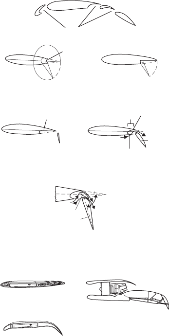
157 Aircraft design and construction

Terminology

Main aerofoil

Slot

Slat

Flap

Vane

Plain flap

Split flap

S

Shroud lip

Shroud

Airflow

through slot

Fowler flap

Single slotted flap

δf

Foreflap

Mainflap

Double slotted flap

High velocity air stream

sticks to sur

face and

changes the lift characteristic

shape

Airfoil 'flexes' to change

Upper surface blowing

'Mission adaptive' wing

Fig. 10.3 Types of flaps

10.1.4 Ground service capability

Fuselage design is influenced by the ground

servicing needs of an aircraft. Ground servicing

represents commercial ‘downtime’ so it is

essential to ensure that as many as possible of

the ground servicing activities can be carried

158 Aeronautical Engineer’s Data Book

Typical Boeing 737/757

Typical Airbus A320

18 in

59 in

84 in

3

per seat

3

per seat

62 in

44.1 in

49.8 in

148 in

49.2 in

56.3 in

155.5 in

1.8 ft

19 in

84 in

2.1 ft

Typical A320 cabin layouts

27

i

n 25

i

n

A

G

1

G

2

G

3

G

4

i

n

coats

57 in

16 first (36 in pitch) + 30 business (36 in pitch)

+ 89 economy (32 in pitch)

72 in 62 in 19

Fig. 10.4 Civil airliner cabin variants

out simultaneously, i.e. the service vehicles and

facilities do not get in each others’ way. Figure

10.5 shows a general arrangement.

10.1.5 Fuselage construction

Most aircraft have either a monocoque or semi-

monocoque fuselage design and use their outer

skin as an integral structural or load carrying

member. A monocoque (single shell) structure

is a thin walled tube or shell which may have

stiffening bulkheads or formers installed

159 Aircraft design and construction

Electrical

power

Bulk cargo

belt loader Fuel truck

Galley/cabin

service

Bulk cargo train

Lavator

y

Galley/cabin

service

Tow

tractor

Portable

Passenger boarding

Lavatory

water truck

bridge

service

Engine

Ground air

air start conditioning

Fig. 10.5 Airliner ground services

within. The stresses in the fuselage are trans-

mitted primarily by the shell. As the shell

diameter increases to form the internal cavity

necessary for a fuselage, the weight-to-strength

ratio changes, and longitudinal stiffeners are

added. This progression leads to the semi-

monocoque fuselage design which depends

primarily on its bulkheads, frames and formers

for vertical strength, and longerons and

stringers for longitudinal strength. Light

general aviation aircraft nearly all have

‘stressed-skin’ construction. The metal skin

exterior is riveted, or bolted and riveted, to the

finished fuselage frame, with the skin carrying

some of the overall loading. The skin is quite

strong in both tension and shear and, if stiff-

ened by other members, can also carry limited

compressive load.

10.1.6 Wing construction

General aviation aircraft wings are normally

either strut braced or full cantilever type,

depending on whether external bracing is used

to help transmit loads from the wings to the

fuselage. Full cantilever wings must resist all

Table 10.3 Indicative material properties: metallic alloys

Yield strength Ultimate tensile strength Modulus Density

R

m

MN/m

2

F

tu

ksi R

m

MN/m

2

F

tu

ksi E GN/m

2

E

t

psi  10

6

 kg/m

3

e

w

lb/in

3

Stainless steel

15–5 PH forgings 1172.2 170 1310 190 196.5 28.5 7833.44 0.283

17–4 PH sheet 724 105 930.8 135 7861.12 0.284

Alloy steel

4130 sheet, plate and tube 517.1 75 655 95 200 29 7833.44 0.283

4330 wrought 1282.5 186 1516.9 220 200 29 7833.44 0.283

4340 bar, tube and forging 1482.4 215 1792.7 260 200 29 7833.44 0.283

Heat-resistant steel

INCONEL 600 sheet, plates, tubes, forgings 206.9 30 551.6 80 206.8 30 8304 0.3

INCONEL 718 sheet plate and tube 999.8 145 1172.1 170 200 29 8304 0.3

Aluminium alloy

2024-T351 plate 282.7 41 393 57 73.8 10.7 2768 0.1

2024-T4 extrusion 303.4 44 413.7 60 73.8 10.7 2768 0.1

2104-T6 forgings 379.2 55 448.2 65 73.8 10.7 2768 0.1

356-T6 castings 137.9 20 206.9 30 71.7 10.4 2684.96 0.097

Titanium alloy

6Al–4V sheet, strip plate 999.8 145 1103.2 160 110.3 16 4428.8 0.16

6Al–6V–2Sn forgings 965.3 140 1034.2 150 117.2 17 4539.52 0.164

160

Table 10.4 Indicative material properties: composites

Ultimate tensile Ultimate compressive Density Maximum service

strength strength temperature

Material R

m

MN/m

2

F

tu

ksi R

c

MN/m

2

F

cu

ksi  kg/m

3

e

w

lb/in

3

°C °F

High temperature 482.6 70 489.5 71 1826.88 0.066 177 350

epoxy fibreglass

Phenolic fibreglass 303.4 44 310.3 45 1826.88 0.066 177 350

Epoxy/graphite 551.6 80 586.1 85 1605.44 0.058 177 350

cloth-woven graphite

Epoxy/Kevlar cloth 496.5 72 193.1 28 1439.36 0.052 177 350

BMI/graphite 648.1 94 730.9 106 1522.4 0.055 232 450

Polymide graphite 730.9 106 717.1 104 1605.44 0.058 315 600

161

Table 10.5 General stainless steels – basic data.

Stainless steels are commonly referred to by their AISI equivalent classification (where applicable)

AISI Other classifications Type

2

Yield F

ty

[(R

e

) MPa] Ultimate [(R

m

) MPa] E(%) HRB %C %Cr % others

1

(ksi) F

tu

(ksi) 50 mm

302 ASTM A296 Austenitic 40 [275.8] 90 [620.6] 55 85 0.15 17–19 8–10 Ni

(cast), Wk 1.4300,

18/8, SIS 2331

304 ASTM A296, , Austenitic 42 [289.6] 84 [579.2] 55 80 0.08 18–20 8–12 Ni

Wk 1.4301, 18/8/LC

SIS 2333, 304S18

304L ASTM A351, , Austenitic 39 [268.9] 80 [551.6] 55 79 0.03 18–20 8–12 Ni

Wk 1.4306 18/8/ELC

SIS 2352, 304S14

316 ASTM A296, Austenitic 42 [289.6] 84 [579.2] 50 79 0.08 16–18 10–14 Ni

Wk 1.4436 18/8/Mo,

SIS 2243, 316S18

316L ASTM A351, Austenitic 42 [289.6] 81 [558.5] 50 79 0.03 16–18 10–14 Ni

Wk 1.4435, 18/8/Mo/ELC,

316S14, SIS 2353

162

321 ASTM A240, Austenitic 35 [241.3] 90 [620.6] 45 80 0.08 17–19 9–12 Ni

Wk 1.4541, 18/8/Ti,

SIS 2337, 321S18

405 ASTM A240/A276/ Ferritic 40 [275.8] 70 [482.7] 30 81 0.08 11.5-14.5 1 Mn

A351, UNS 40500

430 ASTM A176/A240/ Ferritic 50 [344.7] 75 [517.1] 30 83 0.12 14–18 1 Mn

A276, UNS 43000,

Wk 1.4016

403 UNS S40300, ASTM

A176/A276

Martensitic 40 [275.8] 75 [517.1] 35 82 0.15 11.5–13 0.5 Si

410 UNS S40300, ASTM Martensitic 40 [275.8] 75 [517.1] 35 82 0.15 11.5-13.5 4.5–6.5 Ni

A176/A240,

Wk 1.4006

– 255 (Ferralium) Duplex 94 [648.1] 115 [793] 25 280 HV 0.04 24–27 4.5–6.5 Ni

– Avesta SAF 2507

3

, ‘Super’ Duplex 99 [682.6] 116 [799.8]  25 300 HV 0.02 25 7 Ni, 4 Mo,

UNS S32750 40% ferrite 0.3 N

1

Main constituents only shown.

2

All austenitic grades are non-magnetic, ferritic and martensitic grades are magnetic.

3

Avesta trade mark.

163

164 Aeronautical Engineer’s Data Book

loads with their own internal structure. Small,

low speed aircraft have straight, almost rectan-

gular, wings. For these wings, the main load is

in the bending of the wing as it transmits load

to the fuselage, and this bending load is carried

primarily by the spars, which act as the main

structural members of the wing assembly. Ribs

are used to give aerodynamic shape to the wing

profile.

10.2 Materials of construction

The main structural materials of construction

used in aircraft manufacture are based on

steel, aluminium, titanium and composites.

Modern composites such as carbon fibre are in

increasing use as their mechanical and temper-

ature properties improve. Tables 10.3 and 10.4

show indicative information on the properties

of some materials used. Advanced composites

can match the properties of alloys of

aluminium and titanium but are approxi-

mately half their weight. Composite material

specifications and performance data are

manufacturer specific, and are highly variable

depending on the method of formation and

lamination. Composite components in

themselves are costly to manufacture but

overall savings are generally feasible because

they can be made in complex shapes and

sections (i.e. there are fewer components

needing welding, rivets etc.). Some aircraft

now have entire parts of their primary struc-

ture made of carbon fibre composite. Stainless

steel is used for some smaller and engine

components. Table 10.5 gives basic data on

constituents and properties.

10.2.1 Corrosion

It is important to minimize corrosion in

aeronautical structures and engines. Galvanic

corrosion occurs when dissimilar metals are in

contact in a conducting medium. Table 10.6

shows the relative potentials of pure metals.

165 Aircraft design and construction

Table 10.6 The electrochemical series

Gold (Au) + volts

Platinum

(Pt)

Silver (Ag) Noble metals (cathodic)

Copper (Cu)

Hydrogen (H) Reference potential 0 volts

Lead (Pb)

Tin (Sn)

Nickel (Ni)

Cadmium (Cd)

Iron (Fe)

Chromium (Cr) Base metals (anodic)

Zinc (Zn)

Aluminium (Al)

Magnesium (Mg)

Lithium (Li) – Volts

Metals higher in the table become cathodic and are protected by

the (anodic) metals below them in the table.

10.3 Helicopter design

10.3.1 Lift and propulsion

Helicopters differ from fixed wing aircraft in

that both lift and propulsion are provided by a

single item: the rotor. Each main rotor blade

acts as slender wing with the airflow producing

a high reduction in pressure above the front of

the blades, thereby producing lift. Although of

high aspect ratio, the blades are proportion-

ately thicker than those of fixed wing aircraft,

and are often of symmetric profile. Figure 10.6

shows the principle of helicopter airfoil opera-

tion.

10.3.2 Configuration

Figure 10.7 shows the four main configurations

used. The most common is the single main and

tail rotor type in which the torque of the main

rotor drive is counteracted by the lateral force

produced by a horizontal-axis tail rotor. Twin

tandem rotor machines use intermeshing,

counter-rotating rotors with their axes tilted off

the vertical to eliminate any torque imparted to

the helicopter fuselage. In all designs, lift force

is transmitted through the blade roots via the

166 Aeronautical Engineer’s Data Book

Blade

chord line

Relative

wind

Relative wind

Angle of

attack

Lift Resultant

Axis of

rotation

Drag

Fuselage nose down

Angle of

pitch

Tip-path plane

Axis of rotation

Fig. 10.6 Helicopter principles: lift and propulsion

rotor hub into the main drive shaft, so the

helicopter effectively hangs on this shaft.

10.3.3 Forward speed

The performance of standard helicopters is

constrained by fixed design features of the rotat-

ing rotor blades. In forward flight, the ‘retreat-

ing’ blade suffers reversed flow, causing it to lose

lift and stall when the forward speed of the

helicopter reaches a certain value. In addition

the tip speed of the advancing blades suffers

shock-stalls as the blades approach sonic veloc-

ity, again causing lift problems. This effectively

limits the practical forward speed of helicopters

to a maximum of about 310 km/h (192 mph).

10.3.4 Fuel consumption

Helicopters require a higher installed power

per unit of weight than fixed wing aircraft. A

large proportion of the power is needed simply

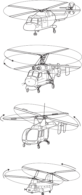
167 Aircraft design and construction

Single main and tail rotor

(general purpose helicopter)

(shipboard helicopter)

C

rotors

Twin co-axial rotors

ounter-rotating

Twin intermeshing rotors

Inclined shaft

(transport helicopter)

meshing rotors

Twin tandem rotors

Counter-rotating

Fig. 10.7 Helicopter configurations

to overcome the force of gravity, and overall

specific fuel consumption (sfc) is high. Figure

10.8 shows how sfc is gradually being reduced

in commercial helicopter designs.

168 Aeronautical Engineer’s Data Book

Specific fuel consumption (sfc) lb/SHP hr

0.8

0.7

0.6

0.5

1950 60 70 80 90 2000

Year

Fig. 10.8 Helicopter sfc trends

10.3.5 Propulsion

Most helicopters are powered either by a single

piston engine or by one, two or three gas

turbine turboshaft engines. A typical gas

turbine model of 1343 kW (1800 hp) comprises

centrifugal and axial compressor stages and two

stage ‘free power’ turbine. The largest units in

use are the 8500 kW+ (11400 hp+) ‘Lotarev’

turboshafts used to power the Mil-26 heavy

transport helicopter. Table 10.7 shows compar-

ative data from various manufacturers’ designs.

10.4 Helicopter design studies

Helicopter design studies follow the general

pattern shown in Figure 10.9. The basis of the

procedure is to start with estimates of gross

weight and installed power based on existing

helicopter designs. First estimates also have to

be made for disc loading and forward flight

drag. The procedure is then interative (as with

the fixed wing design study outlined in Chapter

9) until a design is achieved that satisfies all the

design requirements.

169 Aircraft design and construction

Estimate

gross weight

power

Mission time Fuel capacity

Compare

Payload and crew weights

Check gross

weight

First estimate of disc loading

Main rotor tip

speed

Check

First estimate of for

ward flight drag

Speed and climb

per

formance

requirements

Installed

power

Select engine(s)

Recalculate fuel requirement

Fig. 10.9 Helicopter design studies: the basic steps

10.4.1 Helicopter operational profile

For military helicopters, the operational profile

is frequently termed mission capability. The

relatively short range and low endurance of a

helicopter, compared to fixed wing aircraft,

means that the desired mission profile has a

significant influence on the design. Figure 10.10

shows a typical military mission profile.

Table 10.7 Helicopter comparisons

Model Type Entered Engines Weight Performance

service

No. Type Power Empty Max. Max. speed Max. rate

(each) loaded

at sea level of climb

Aerospatiale

SA 330 Puma

Agusta A129

Mangusta

Bell Huey

AH–1 Cobra

Eurocopter

UHU/HAC

Kamov Ka–50

Medium transport

Attack helicopter

Anti-tank

helicopter

Close-support

helicopter

1965

1983

1965

1991

1982

2 Turbomeca

turboshaft

2 GEM 2

turboshaft

1 turboshaft

2 MTR

turboshaft

2 Klimov

turboshaft

991 kW

(1328 hp)

708 kW

(952 hp)

1044 kW

(1400 hp)

1160 kW

(1556 hp)

1634 kW

(2190 hp)

3536 kg

(7795 lb)

2529 kg

(5575 lb)

2755 kg

(6073 lb)

3300 kg

(7275 lb)

4550 kg

(10 030 lb)

6400 kg

(14 110 lb)

4100 kg

(9039 lb)

4310 kg

(9500 lb)

5800 kg

(12 787 lb)

10 800 kg

(23 810 lb

280 km/h

(174 mph)

259 km/h

(161 mph)

277 km/h

(172 mph

280 km/h

(174 mph)

310 km/h

(193 mph)

366 m/min

(1200 ft/min)

637 m/min

(2090 ft/min)

375 m/min

(1230 ft/min)

600 m/min

(1970 ft/min)

600 m/min

(1970 ft/min)

Mil Mi–26 Heavy transport

helicopter

1979 2 Lotaren

turboshaft

8504 kW

(11 400 hp)

28 200 kg

(62 169 lb)

49 500 kg

(10 9127 lb)

295 km/h

(183 mph)

–

Boeing CH–47

Chinook

Medium transport

helicopter

1961 2 Allied signal

turboshaft

1641 kW

(2200 hp)

9242 kg

(20 378 lb)

20 866 kg

(46 000 lb)

306 km/h

(190 mph)

878 m/min

(2880 ft/min)

Bell/Boeing

V–22 Osprey

Multi-role VTOL

rotorcraft

1989 2 Allison

turboshaft

4588 kW

(6150 hp)

14 800 kg

(32 628 lb)

VTOL:

21546 kg

(47 500 lb)

STOL:

629 km/h

(391 mph)

–

24 948 kg

(5500 lb)

EH101 Merlin Multi-role

helicopter

1987 3 GE turboshaft 1522 kW

(2040 hp)

9072 kg

(20 000 lb)

14 600 kg

(32 188 lb)

309 km/h

(192 mph)

–

172 Aeronautical Engineer’s Data Book

Cruise to target zone

Engage target

Return to base with fuel

reserve

Descend and hide

Climb to cruise

Fig. 10.10 Typical military helicopter ‘mission profile’

Section 11

Airport design and compatibility

Airports play an important role in the civil and

military aeronautical industries. They are part

of the key infrastructure of these industries

and, because of their long construction times

and high costs, act as one of the major fixed

constraints on the design of aircraft.

11.1 Basics of airport design

11.1.1 The airport design process

The process of airport design is a complex

compromise between multiple physical,

commercial and environmental considerations.

Physical facilities needed include runways,

taxiways, aprons and strips, which are used for

the landing and take-off of aircraft, for the

manoeuvring and positioning of aircraft on the

ground, and for the parking of aircraft for

loading and discharge of passengers and cargo.

Lighting and radio navigation are essential for

the safe landing and take-off of aircraft. These

are supplemented by airfield markings, signals,

and air traffic control facilities. Support facili-

ties on the airside include meteorology, fire

and rescue, power and other utilities, mainte-

nance, and airport maintenance. Landside

facilities are the passenger and cargo terminals

and the infrastructure system, which includes

parking, roads, public transport facilities, and

loading and unloading areas. At all stages of

the design process, the issue of aircraft compat-

ibility is of prime importance – an airport must

be suitable for the aircraft that will use it, and

vice versa.

174 Aeronautical Engineer’s Data Book

11.1.2 Airport site selection

The airport site selection process includes

several stages of activity. Table 11.1 shows the

main ‘first stage balance factors’.

Table 11.1 Airport site selection: ‘first stage balance factors’

Aeronautical requirements Environmental constraints

• Flat area of land (up to • Should not impinge on

3000* acres for a large areas of natural beauty

facility) • Sufficiently far away

• Sufficiently close to

population centres to

allow passenger access

from urban centres to

minimize the adverse

effects of noise etc.

*Note: Some large international airports exceed this figure (e.g.

Jeddah, Saudi Arabia and Charles de Gaulle, Paris).

11.1.3 Operational requirements – ‘rules of thumb’

There is a large variation in the appearance and

layout of airport sites but all follow basic ‘rules

of thumb’:

• The location and orientation of the runways

are primarily decided by the requirement to

avoid obstacles during take-off and landing

procedures. 15

km is used as a nominal

‘design’ distance.

• Runway configuration is chosen so that they

will have manageable crosswind compo-

nents (for the types of aircraft being used)

for at least 95% of operational time.

• The number of runways available for use at

any moment determines the

operational

capacity of the airport. Figure 11.1 shows

common runway layouts. Crosswind facility

is achieved by using either a ‘crossed’ or

‘open or closed vee’ layout.

• Operational capacity can be reduced under

IFR (Instrument Flying Rules) weather

conditions when it may not be permissible

to use some combinations of runways simul-

taneously unless there is sufficient separa-

tion (nominally 1500+ metres).

175 Airport design and compatibility

(a) Close parallel runways

< 500 m

(b) Independent parallel runways

(c) Crossed runways

> 1500 m

(d) 'Closed-vee' runways

Fig. 11.1 Common runway layouts

176 Aeronautical Engineer’s Data Book

Fig. 11.2 Birmingham airport – a crossed runway layout

177 Airport design and compatibility

Figure 11.2 shows Birmingham (UK) airport

layout – a mid-size regional airport with crossed

runway design. Figure 11.3 shows a large

national airport with a crossed and indepen-

dent parallel runway layout.

Fig. 11.3 A crossed and independent parallel runway

layout

11.1.4 Aircraft:airport compatibility

A prime issue in the design of a new airport, or

the upgrading of an existing one, is

aircraft:airport compatibility. Aircraft and

airport design both have long lead times, which

means that new airports have to be designed to

meet the constraints of existing and planned

aircraft designs, and vice versa. These

constraints extend across the various elements

of airport design, i.e. runway length, width and

178 Aeronautical Engineer’s Data Book

Aircraft design

Ground

manoeuvring

landing runs

Ground

pavement strength

Door

clearances

Clearance

radii

Landing gear

footprint

Airport design

Take-off and

servicing

Take-off/landing

/taxi loads v.

Turn

geometry

Fig. 11.4 Aircraft:airport compatibility – some important

considerations

orientation, taxiways and holding bays,

pavement design, ground servicing arrange-

ments and passenger/cargo transfer facilities.

Figure 11.4 shows a diagrammatic representa-

tion of the situation.

Details of aircraft characteristics are

obtained from their manufacturers’ manuals,

which address specifically those characteristics

which impinge upon airport planning. The

following sections show the typical format of

such characteristics, using as an example the

Boeing 777 aircraft.

General dimensions

The general dimensions of an aircraft have an

influence on the width of runways, taxiways,

holding bays and parking bays. Both wingspan

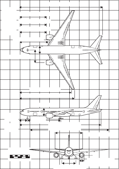
179 Airport design and compatibility

209 ft 1 in (63.73m)

66 ft 0.5 in (20.13m)

67 ft 0 in (20.42m)

70 ft 9.5 in (21.58m)

20 ft 4 in (6.2m)

31 ft 6.5 in (9.61m)

131 ft 0 in (39.94 m)

138 ft 0 in (42.06 m)

20 ft 4 in (6.2 m)

206 ft 6 in (62.94 m)

199 ft 11 in (60.93 m)

70 ft 7.5 in (21.53 m)

36 ft 0 in (10.97 m)

13 ft 0 in (3.96 m)

nominal

19 ft 4 in

(5.89 m)

19 ft 4 in

(5.89 m)

84 ft 11 in

25.88 m)

66 ft 4.0 in (20.22m)

engine)

(PW4074

engine)

(GE 90B3

engine)

SCALE

Meters

Feet

0 2 4 6 8

50403020100

(Trent870

10 12 14

Fig. 11.5 Aircraft:airport compatibility – general

dimensions. Figure shows Boeing 777-200. Courtesy

Boeing Commercial Airplane Group

and overall length can place major constraints

on an airport’s design. Figure 11.5 shows typical

data.

General clearances

Aircraft ground clearance is an important crite-

rion when considering ground-based obstacles

and both fixed and mobile ground servicing

facilities. Figure 11.6 shows typical data.

Door location and type

The location and type of doors have an influ-

ence on passenger access and cargo handling

design aspects of the overall airport facility.

180 Aeronautical Engineer’s Data Book

A B C D E F J KG L H

Minimum* Maximum*

Feet - inches Meters Feet - inches Meters

A 27-6 8.39 28-6 8.68

B 15-5 4.71 16-5 5.00

C 9-3 2.81 10-0 3.05

D 16-0 4.88 16-7 5.07

E (PW) 3-2 0.96 3-5 1.04

E (GE) 2-10 0.85 3-1 0.93

E (RR) 3-7 1.09 3-10 1.17

F 16-10 5.14 17-4 5.28

G (Large door) 10-7 3.23 11-2 3.41

G (Small door) 10-6 3.22 11-2 3.40

H 10-7 3.23 11-5 3.48

J 17-4 5.28 18-2 5.54

K 60-5 18.42 61-6 18.76

L 23-6 7.16 24-6 7.49

Fig. 11.6 Aircraft:airport compatibility – ground

clearances. Figure shows Boeing 777-200. Courtesy

Boeing Commercial Airplane Group

Figures 11.7 and 11.8 show typical passenger

door locations and clearances. Figures 11.9 and

11.10 show comparable data for cargo doors.

162 ft 6 in (49.54 m)

119 ft 2 in (36.33 m)

56 ft (17.07 m)

22 ft 1.5 in

(6.75 m)

Fig. 11.7 Aircraft:airport compatibility – passenger door

locations. Figure shows Boeing 777-200. Courtesy Boeing

Commercial Airplane Group

181 Airport design and compatibility

4 ft 1 in (1.25 m)

2 ft 7 in

(0.78 m)

2 ft 9 in

(0.84 m)

2 ft 4 in

(0.72 m)

INBD

2.34 in

(0.006 m)

FWD

7 ft 11 in (2.42 m)

3 in overlift (2)

FWD

Door sill

Outside of door 1

2 in 1

(left door shown, right door oposite)

Notes:

(1) Door moves up 2 in. and inward 0.4 in. to clear stops

before opening outward

(2) Door capable of moving an additional 3 in vertically (overlift)

to preclude damage from contact with loading bridge

Fig. 11.8 Aircraft:airport compatibility – passenger door

clearances. Figure shows Boeing 777-200. Courtesy

Boeing Commercial Airplane Group

151 ft 11.5 in (46.2 m)

136 ft 9.5 in (41.7 m)

136 ft 4 in (41.3 m)

clear opening

106 by 67 in

(2.7 by 1.7 m)

38 ft 8.5 in

(11.9 m)

Aft cargo door

clear opening 70 by 67 in

(1.8 by 1.7 m)

Optional aft cargo door

clear opening 106 by 67 in

(2.7 by 1.7 m)

Bulk cargo door

clear opening

36 by 45 in

(0.9 by 1.1 m)

Forward cargo door

Fig. 11.9 Aircraft:airport compatibility – cargo door

locations. Figure shows Boeing 777-200. Courtesy Boeing

Commercial Airplane Group

182 Aeronautical Engineer’s Data Book

Airplane

17 ft 7 in (5.36 m)

Large cargo door

open position

Sidewall

3 in (7.6 m)

Ceiling

2 in (5 cm)

LD-3 5 ft 7 in (1.70 m)

container

5 ft 4 in

clear opening

(1.62 m)

18 ft 1 in (5.52 m) max

17 ft 2 in (5.23 m) min

Container

View looking forward

Door

Ground line

open

1 ft 5 in (0.43 m)

Door

clear

Cargo handling

8 ft 10 in

control panel

opening

(2.69 m)

5 ft 7 in

1 ft 4 in (0.41 m)

Cargo door actuation

(1.70 m)

panel

13 ft 5 in (4.10 m) max

12 ft 6 in (3.81 m) min

FWD

11 ft 4 in (3.46 m) max

10 ft 5 in (3.17 m ) min

View looking inboard

Ground line

Fig. 11.10 Aircraft:airport compatibility – cargo door

clearances. Figure shows Boeing 777-200. Courtesy

Boeing Commercial Airplane Group

Runway take-off and landing length

requirements

Every aircraft manual contains runway length

requirements for take-off and landing. A series

of characteristic curves are provided for various

pressure altitudes (i.e. the airport location

above sea level), ambient temperature aircraft

weights, wind, runway gradient and conditions

etc. Figures 11.11 and 11.2 show typical data,

and the way in which the graphs are presented.

Manoeuvring geometry and clearances

Aircraft turn radii and clearances can influence

the design of taxiways, holding bays intersections

etc. as well as parking bays and manoeuvring

183 Airport design and compatibility

Notes:

• Consult using airline for specific operating procedure prior to facility design

• Zero runway gradient

• Zero wind

Pressure altitude

Feet Meters

FAR landing runway length (1,000 meters)

2.50

8

2.25

7

2.00

1.75

1.50

1.25

5

6

1,000 Feet

10,000

8,000

6,000

4,000

2,000

(3,049

(2,439)

(1,829)

(1,219)

(609)

Sea level

Dry runway

Wet runway

4

1.00

3

300 320 340 360 380 400 420 440 460

1,000 pounds

140 150 160 170 180 190 200 210

(1,000 kilograms) operational landing weight

Fig. 11.11 Aircraft:airport compatibility – landing

runway length requirements. Figure shows Boeing 777-

200. Courtesy Boeing Commercial Airplane Group

Notes:

• Consult using airline for specific operating procedure prior to facility design

• Air conditioning off

• Zero runway gradient

• Zero wind

F.A.R. Takeoff runway length (1,000 meters)

4.5

4.0

3.5

3.0

2.5

2.0

1.5

1.0

15

14

13

12

11

10

9

8

7

6

5

4

3

Standard ayd

Flap 5

Flap 15

altitude

ers)

Flap 20

F

Pres

eet

9,000

su

re

(2,

(met

743)

8,000

6,000

(2

(

,438)

1,829)

9)

4,000

2,000

(1,21

(610)

M

54

axi

5,000

mu

LB

m takeoff eiw ght

)

Sea level

(247,300 kg

340 360 380 400 420 440 460 480 500 520 540 560 580

1,000 pounds

160 170 180 190 200 210 220 230 240 250 260

(1,000 kilograms) Brake-release gross weight

Fig. 11.12 Aircraft:airport compatibility – take-off

runway length requirements. Figure shows Boeing 777-

200. Courtesy Boeing Commercial Airplane Group

184 Aeronautical Engineer’s Data Book

Steering

angle

Notes:

• Data shown for airplane with aft axle steering

• Actual operating turning radii may be greater than shown.

R1

R5

R3

R2

R4

R6

45°

50°

55°

60°

65°

Nose gear axle

projection

Main gear

centreline projection

(typical for steering

angles shown)

24 in (0.61 m)

Turning centre

• Consult with airline for specific operating procedure

• Dimensions rounded to nearest foot and 0.1 meter

Steering R1 R2 R3

angle Inner Outer Nose

gear gear gear

(Deg) Ft M Ft M Ft M

30 123 37.5 165 50.3 168 51.3

35 98 29.7 140 42.6 147 44.8

40 78 23.7 120 36.6 131 40.0

45 62 18.9 104 31.7 120 36.4

50 49 14.8 91 27.7 111 33.7

55 37 11.2 79 24.1 103 31.5

60 27 8.1 69 21.0 98 29.9

65 17 5.3 60 18.2 94 28.6

70 (max) 9 2.7 51 15.6 90 27.6

R4 R5 R6

Wing tip Nose Tail

Ft M Ft M Ft M

247 75.3 177 53.8 209 63.6

222 67.6 157 47.8 187 57.1

202 61.7 142 43.4 171 52.2

187 56.9 132 40.2 159 48.5

174 52.9 124 37.7 150 45.6

162 49.5 118 35.8 142 43.2

152

46.5 113 34.4 135 41.2

143 43.7 109 33.3 130 39.5

135 41.2 107 32.5 125 38.1

Fig. 11.13 Aircraft:airport compatibility – turning radii.

Figure shows Boeing 777-200. Courtesy Boeing

Commercial Airplane Group

185 Airport design and compatibility

capabilities in the vicinity of passenger and cargo

loading facilities. Different types and sizes of

aircraft can have very different landing gear

tracks and ‘footprints’ – hence an airport’s design

often has to incorporate compromises, so that it

is suitable for a variety of aircraft types. Figure

11.13 shows the typical way that turn radii are

64°

X Y

70°

max

2ft (0.61 m)

A

Minimum pavement width

for 180° turn

(outside to outside of tire)

For planning width

consult using airlines

Theoretical centre of turn

R6 – Tail

R5 – Nose

R4 – Wingtip

R3 – Nose gear

for minimum turning radius.

Slow continuous turn with

differential thrust.

Notes: 1.

6° Tire slip angle approximate

No differential braking

for 64 turn angle.

2. Consult using airline for specific operating procedure.

3. Dimensions are rounded to the nearest foot and 0.1 meter.

Airplane Effective

model steering

angle (Deg)

X Y A R3

777-200

777-300

64

FT

83

100

M

5.3

30.6

FT

40

49

M

12.2

14.9

FT

156

182

M

47.5

55.4

FT

95

112

M

29.0

34.0

R4 R5 R6

FT M FT M FT M

145 44.2 110 33.5 131 39.9

154 46.8 129 39.4 149 45.3

Fig. 11.14 Aircraft:airport compatibility – clearance

radii. Figure shows Boeing 777-200. Courtesy Boeing

Commercial Airplane Group

186 Aeronautical Engineer’s Data Book

expressed. Figure 11.14 shows corresponding

clearance radii and the way in which the aircraft

characteristics for a 180° turn define the

minimum acceptable pavement width that is

necessary.

150ft (45 m)

80ft (24 m)

75ft

(23 m)

150ft

of outboard wheel

Centreline of runway

Additional fillet

as required for

edge margin

FAA lead-in fillet

Track of outside edge

(45 m)

Fig. 11.15 Aircraft:airport compatibility – runway and

taxiway intersections (> 90°). Figure shows Boeing 777-

200/300. Courtesy Boeing Commercial Airplane Group

75 ft

(23 m)

Approx 14 ft

(4 m)

85 ft (26 m)

150 ft (45 m)

of outboard wheel

Centreline of runway

150 ft (45 m)

FAA lead-in fillet

Track of outside edge

Fig. 11.16 Aircraft:airport compatibility – runway and

taxiway intersections (90°). Figure shows Boeing 777-

200/300. Courtesy Boeing Commercial Airplane Group

187 Airport design and compatibility

Shoulder

317 ft

(96.6 m)

20 ft

40 ft

(6.2 m)

75ft (23 m)

20 ft (6.1 m) clearance

between centreline of gear

and pavement edge

Note

Before determining the size of the

intersection fillet, check with the

airlines regarding the operating

procedures that they use and the

To

runway

aircraft types that are expected

to serve the airport

Fig. 11.17 Aircraft:airport compatibility – holding bay

sizing. Figure shows Boeing 777-200/300. Courtesy Boeing

Commercial Airplane Group

An important aspect of aircraft:airport

compatibility is the required geometry of

runway and taxiway turnpaths and intersec-

tions. Consideration must be given to features

such as intersection fillets, sized to accommo-

date aircraft types expected to use the airport.

Figures 11.15 and 11.16 show typical character-

istics for 90° and > 90° turnpaths. Figure 11.17

shows a corresponding holding bay arrange-

ment – note the need for adequate wing tip

clearance between holding aircraft, and clear-

ance between each aircraft’s landing gear track

and the pavement edge.

Pavement strength

Airports’ pavement type and strength must be

designed to be compatible with the landing gear

loadings, and the frequency of these loadings, of

the aircraft that will use it. A standardized

188 Aeronautical Engineer’s Data Book

Notes:

* Tires – 50 x 20 R22 32 PR

* Pressure – 215 PSI (15.12 KG/CM SQ)

100

80

60

40

20

0

Notes:

1. ACN was determined as referenced in

ICAQ aerodrome design manual part 3,

part 1.1, second edition, 1983

2. determine main landing gear loading,

see sction 7.4.

3.

Code D – k = 75 (ultra low)

Code C – k = 150 (low)

Code B – k =300 (medium)

Code A – k = 550 (high)

Aircraft classification number (ACN)

To

Percent weight on mainn landing gear: 93.8

300 350 400 450 500 550 600 650 700

1,000 LB

150 200

250 300

(1,000 Kg)

Aircraft gross weight

Fig. 11.18 Aircraft:airport compatibility – aircraft

classification No.: rigid pavement. Data for Boeing 777-

200. Courtesy Boeing Commercial Airplane Group

compatibility assessment is provided by the

Aircraft Classification Number/Pavement

Classification Number (ACN/PCN) system. An

aircraft having an ACN equal to or less than the

pavement’s PCN can use the pavement safely, as

long as it complies with any restrictions on the

tyre pressures used. Figures 11.18 and 11.19

show typical rigid pavement data (see also

Section 11.2) whilst Figure 11.20 shows data for

flexible pavement use.

Airside and landside services

The main airside and landside services consid-

ered at the airport design stage are outlined in

Table 11.2.

11.1.5 Airport design types

The design of an airport depends principally on

the passenger volumes to be served and the

type of passenger involved. Some airports have

a very high percentage of passengers who are

transiting the airport rather than treating it as

their final destination, e.g. Chicago O’Hare

189 Airport design and compatibility

Note: All tires – all contact area constant at 243 Sq in (0.157 Sq M)

Weight on main gear

900

627,700 LB

(284,800 KG)

600,000 LB

K =

k =

75

150

300

k = 550

60

850

(272,200 KG)

550,000 LB

Flexural strength ( KG/SQ CM) Flexural strength ( KG/SQ CM)

800

(249,550 KG)

55

750

500,000 LB

(226,850 KG)

50

PSI PSI

700

450,000 LB

(204,150 KG)

400,000 LB

650

45

40

35

60

55

50

(181,450 KG)

350,000 LB

600

(150,800 KG)

550

500

900

850

800

750

700

650

Annual dep

1,2

3,0

artu

00

res

6,0

15,0

25,0

00

N

pavem

ote:

ent

200-

life

yer

C:/R13/WIN/777APD/SEC79/SEC79.DWG

45

600

40

550

35

500

6 81

0 12 14 1618 20 22 24

Inches

20 30 40 50 60

(Centimeters)

Pavement thickness

Fig. 11.19 Aircraft:airport compatibility – rigid

pavement requirements. Data for Boeing 777-200.

Courtesy Boeing Commercial Airplane Group

190 Aeronautical Engineer’s Data Book

N

otes:

* 50 x 20 R22 32 PR

* Pressure – 215 PSI (15.12 KG/CM SQ)

100

80

60

40

20

0

300 350 400 500 600 700650550450

Notes:

1. ACN was calculated using

alpha factors proposed by the

ICAO ACN study group

2. determine main landing gear loading,

see sction 7.4.

3.

Code D – CBR 3 (ultra low)

Code C – CBR 6 (low)

Code B – CBR 10 (medium)

Code A – CBR 15(high)

Aircraft classification number (ACN)

To

Percent weight on mainn landing gear: 93.8

1,000 LB

150 200

250 300

(1,000 Kg)

Aircraft gross weight

Fig. 11.20 Aircraft:airport compatibility – aircraft

classification No.: flexible pavement. Data for Boeing

777-200. Courtesy Boeing Commercial Airplane Group

International (USA). These are referred to as

hubbing airports. At a hub, aircraft from a

carrier arrive in waves, and passengers transfer

between aircraft during the periods when these

waves are on the ground. By using a hub-and-

spoke design philosophy, airlines are able to

increase the load factors on aircraft and to

provide more frequent departures for passen-

gers – at the cost, however, of inconvenient

interchange at the hub.

11.1.6 Airport capacity

The various facilities at an airport are designed

to cope adequately with the anticipated flow of

passengers and cargo. At smaller single-runway

airports, limits to capacity usually occur in the

terminal areas, since the operational capacity of

a single runway with adequate taxiways is quite

large. When passenger volumes reach approxi-

mately 25 million per year, a single runway is no

longer adequate to handle the number of aircraft

movements that take place during peak periods.

At this point at least one additional runway,

191 Airport design and compatibility

Table 11.2 Airside and landside service considerations

Landside Airside

• Ground passenger • Aircraft apron handling

handling including: • Airside passenger

– Check-in transfer

– Security • Baggage and cargo

– Customs and handling

immigration • Aircraft fuelling

– Information • Cabin cleaning and

– Catering catering

– Cleaning and • Engine starting

maintenance maintenance

– Shopping and • Aircraft de-icing

concessionary facilities • Runway inspection and

– Ground transportation maintenance

• Management and

administration of airport

staff

• Firefighting and

emergency services

• Air traffic control

Other basic airport requirements are:

• Navigation aids – normally comprising an Instrument

Landing System (ILS) to guide aircraft from 15 miles

from the runway threshold. Other commonly installed

aids are:

– Visual approach slope indicator system (VASIS)

– Precise approach path indicator (PAPI)

• Airfield lighting – White neon lighting extending up to

approximately 900 m before the runway threshold,

threshold lights (green), ‘usable pavement end’ lights

(red) and taxiway lights (blue edges and green

centreline).

permitting simultaneous operation, is required.

Airports with two simultaneous runways can

frequently handle over 50 million passengers per

year, with the main constraint being, again, the

provision of adequate terminal space.

Layouts with four parallel runways can have

operational capacities of more than one million

aircraft movements per year and annual

passenger movements in excess of 100 million.

The main capacity constraints of such facilities

are in the provision of sufficient airspace for

controlled aircraft movements and in the provi-

sion of adequate access facilities. Most large

international airport designs face access

problems before they reach the operational

capacity of their runways.

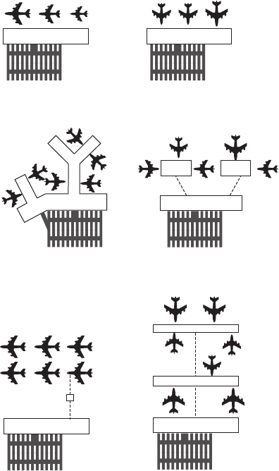
192 Aeronautical Engineer’s Data Book

11.1.7 Terminal designs

Open apron and linear designs

The simplest layout for passenger terminals is the

open apron design

(Figure 11.21(a)) in which

aircraft park on the apron immediately adjacent

to the terminal and passengers walk across the

apron to board the aircraft. Frequently, the

aircraft manoeuvre in and out of the parking

Open apron Linear

building

Parking Parking

building

Terminal Terminal

Pier

Satellite

Parking

building

Terminal

Remote pier

Parking

building

Mobile lounge

(transporter)

building

Terminal

Transporter

Terminal

Transporter

Fig. 11.21 Airport terminal designs

193 Airport design and compatibility

positions under their own power. When the

number of passengers walking across the apron

reaches unmanageable levels the optimum design

changes to the linear type (Figure 11.21(b)) in

which aircraft are parked at gates immediately

adjacent to the terminal itself, and passengers

board by air bridge. The limitation of the linear

concept is usually the long building dimensions

required; this can mean long walking distances for

transferring passengers and other complications

related to building operation. In most designs,

building lengths reach a maximum of approxi-

mately 700 m. Examples are Kansas City Inter-

national, USA, Munich, Germany (Figure 11.22),

and Paris Charles de Gaulle, France.

Pier and satellite designs

The pier concept

(Figure 11.21(c)) has a design

philosophy in which a single terminal building

serves multiple aircraft gates (Frankfurt and

Schipol used this concept prior to their recent

expansion programmes). The natural extension

of this is the satellite concept (Figure 11.21(d)),

in which passengers are carried out to the satel-

lites by automated people-mover or automatic

train. This design is difficult to adapt to the

changing size of aircraft and can be wasteful of

apron space.

Transporter designs

The transporter concept (Figure 11.21(e)) is one

method of reducing the need for assistance for

aircraft manoeuvring on the apron and elimi-

nating the need for passengers to climb up and

down stairways to enter or exit the aircraft.

Passengers are transported directly to the

aircraft by specialized transporter vehicles which

can be raised and lowered (Dulles International,

USA and Jeddah’s King Abdul Aziz Interna-

tional Airport, Saudi Arabia, are examples).

Remote pier designs

In this design (Figure 11.21(f)) passengers are

brought out to a remote pier by an automatic

194

Fig. 11.22 Munich airport layout – a ‘linear’ design

195 Airport design and compatibility

people-mover and embark or disembark in the

conventional manner (Stansted, UK, is an

example).

Unit terminals

The term

unit terminal is used when an airport

passenger terminal system comprises more than

one terminal. Unit terminals may be made up of

a number of terminals of similar design (Dallas-

Fort Worth, USA), terminals of different design

(London Heathrow), terminals fulfilling differ-

ent functions (London Heathrow, Arlanda,

Stockholm), or terminals serving different

airlines (Paris Charles de Gaulle). The success-

ful operation of unit terminal airports requires

rapid and efficient automatic people-movers

that operate between the terminals.

11.1.8 The apron

An important requirement in the design of an

airport is minimizing the time needed to service

an aircraft after it has landed. This is especially

important in the handling of short-haul aircraft,

where unproductive ground time can consume an

unacceptably large percentage of flight time. The

turnaround time for a large passenger transport

between short-haul flights can be as little as 25

minutes. During this period, a large number of

service vehicles circulate on the apron (see Figure

10.5 in Chapter 10), so an important aspect of the

efficient operation of an airport facility is the

marshalling of ground service vehicles and aircraft

in the terminal apron area. Such an operation can

become extremely complex at some of the world’s

busiest international airports, where an aircraft

enters or leaves the terminal apron approximately

every 20 seconds.

11.1.9 Cargo facilities

Although only approximately 1–2% of world-

wide freight tonnage is carried by air, a large

international airport may handle more than one

million tons of cargo per year. Approximately

10% of air cargo is carried loose or in bulk, the

196 Aeronautical Engineer’s Data Book

remainder in air-freight containers. In devel-

oped countries, freight is moved by mobile

mechanical equipment such as stackers, tugs,

and forklift trucks. At high-volume facilities, a

mixture of mobile equipment and complex fixed

stacking and movement systems must be used.

Fixed systems are known as transfer vehicles

(TVs) and elevating transfer vehicles (ETVs).

An area of high business growth is specialized

movement by courier companies which offer

door-to-door delivery of small packages at

premium rates. Cargo terminals for the small-

package business are designed and constructed

separately from conventional air-cargo termi-

nals – they operate in a different manner, with

all packages being cleared on an overnight basis.

11.2 Runway pavements

Modern airport runway lengths are fairly

static owing to the predictable take-off run

requirements of current turbofan civil aircraft.

All but the smallest airports require

pavements for runways, taxiways, aprons and

maintenance areas. Table 11.3 shows basic

pavement requirements and Figure 11.23 the

two common types.

Table 11.3 Runway pavements – basic requirements

• Ability to bear aircraft weight without failure

• Smooth and stable surface

• Free from dust and loose particles

• Ability to dissipate runway loading without causing

subgrade/subsoil failure

• Ability to prevent weakening of the subsoil by rainfall

and frost intrusion

The two main types of pavement are:

• Rigid pavements: Cement slabs over a granular sub-

base or sub-grade. Load is transmitted mainly by the

distortion of the cement slabs.

• Flexible pavements: Asphalt or bitumous concrete

layers overlying granular material over a prepared sub-

grade. Runway load is spread throughout the depth of

the concrete layers, dissipating sufficiently so the

underlying subsoil is not overloaded.

197 Airport design and compatibility

Typical rigid runway pavement

Typical flexible asphalt-based runway pavement

Rigid portland

cement slab

Sub-base

Underlying foundation

Top dressing

Asphalt sur

face

Base course

Sub-base

Underlying foundation

Fig. 11.23 Rigid and flexible runway pavements

11.3 Airport traffic data

Tables 11.4 and 11.5 show recent traffic ranking

data for world civil airports.

11.4 FAA–AAS Airport documents

Technical and legislative aspects of airport design

are complex and reference must be made to up-

to-date documentation covering this subject. The

Office of Airport Safety and Standards (ASS)

serves as the principal organization of United

States Federal Aviation Authority (FAA)

responsible for all airport programme matters

about standards for airport design, construction,

maintenance, operations and safety. References

available are broadly as shown in Table 11.6 (see

also www.faa.gov/arp/topics.htm).

198 Aeronautical Engineer’s Data Book

Table 11.4 World airports ranking by total aircraft

movements - 1999–2000

Rank Airport Total aircraft % change

movements over year

1 Atlanta (ATL) 909 911 7.4

2 Chicago (ORD) 896 228 n.a.

3 Dallas/Ft Worth 831 959 –0.5

airport (DFW)

4 Los Angeles (LAX) 764 653 1.2

5 Phoenix (PHX) 562 714 4.6

6 Detroit (DTW) 559 546 3.8

7 Las Vegas (LAS) 542 922 15.3

8 Oakland (OAK) 524 203 3.5

9 Miami (MIA) 519 861 –3.1

10 Minneapolis/ 510 421 5.7

St Paul (MSP)

11 St Louis (STL) 502 865 –2

12 Long Beach (LGB) 499 090 5.8

13 Boston (BOS) 494 816 –2.5

14 Denver (DEN) 488 201 5.3

15 Philadelphia (PHL) 480 276 2.3

16 Cincinnati 476 128 7.7

(Hebron) (CVG)

17 Paris (CDG) 475 731 10.7

18 Santa Ana (SNA) 471 676 12.9

19 Washington (IAD) 469 086 22.7

20 Houston (IAH) 463 173 3.5

21 London (LHR) 458 270 1.5

22 Newark (EWR) 457 235 0.3

23 Frankfurt/Main (FRA) 439 093 5.5

24 San Francisco (SFO) 438 685 1.5

25 Pittsburgh (PIT) 437 587 –3

26 Seattle (SEA) 434 425 6.6

27 Charlotte (CLT) 432 128 –2.2

28 Toronto (YYZ) 427 315 1

29 Amsterdam (AMS) 409 999 4.4

30 Memphis (MEM) 374 817

199 Airport design and compatibility

Table 11.5 Ranking by passenger throughput

Airport Passenger

throughput

1 Atlanta (ATL) 78 092 940

2 Chicago (ORD) 72 609 191

3 Los Angeles (LAX) 64 279 571

4 London (LHR) 62 263 365

5 Dallas/Ft Worth airport (DFW) 60 000 127

6 Tokyo (HND) 54 338 212

7 Frankfurt/Main (FRA) 45 838 864

8 Paris (CDG) 43 597 194

9 San Francisco (SFO) 40 387 538

10 Denver (DEN) 38 034 017

11 Amsterdam (AMS) 36 772 015

12 Minneapolis/St Paul (MSP) 34 721 879

13 Detroit (DTW) 34 038 381

14 Miami (MIA) 33 899 332

15 Las Vegas (LAS) 33 669 185

16 Newark (EWR) 33 622 686

17 Phoenix (PHX) 33 554 407

18 Seoul (SEL) 33 371 074

19 Houston (IAH) 33 051 248

20 New York (JFK) 31 700 604

21 London (LGW) 30 559 227

22 St Louis (STL) 30 188 973

23 Hong Kong (HKG) 29 728 145

24 Orlando (MCO) 29 203 755

25 Madrid (MAD) 27 994 193

26 Toronto (YYZ) 27 779 675

27 Seattle (SEA) 27 705 488

28 Bangkok (BKK) 27 289 299

29 Boston (BOS) 27 052 078

30 Singapore (SIN) 26 064 645

Source of data: ACI.

200 Aeronautical Engineer’s Data Book

Table 11.6 FAA–AAS airport related documents

• Airport Ground Vehicle Operations Guide

• Airports (150 Series) Advisory Circulars

• Airports (150 Series) Advisory Circulars (Draft)

• 5010 Data (Airport Master Record) AAS-300

• Access for Passengers With Disabilities

• Activity Data

• AIP APP-500

• AIP Advisory Circular List

• AIP Grants Lists APP-520

• AIP Project Lists APP-520

• Aircraft Rescue and Firefighting Criteria AAS-100

• AC 150/5210-13A Water Rescue Plans, Facilities, and

Equipment

• AC 150/5210-14A Airport Fire and Rescue Personnel

Protective Clothing

• AC 150/5210-17 Programs for Training of Aircraft

Rescue and Firefighting Personnel

• AC 150/5210-18 Systems for Interactive Training of

Airport Personnel

• AC 150/5210-19 Driver’s Enhanced Vision System

(DEVS)

• AC 150/5220-4B Water Supply Systems for Aircraft

Fire and Rescue Protection

• AC 150/5220-10B Guide Specification for Water Foam

Aircraft Rescue and Firefighting Vehicles

• AC 150/5220-19 Guide Specification for Small Agent

Aircraft Rescue and Firefighting Vehicles

• Aircraft Rescue and Firefighting Regulations AAS-310

• Aircraft/Wildlife Strikes (Electronic Filing) (AAS-310)

• Airport Activity Data

• Airport Buildings Specifications AAS-100

• AC 150/5220-18 Buildings for Storage and

Maintenance of Airport Snow and Ice Control

Equipment and Materials

• Airport Capacity and Delay AAS-100

• Airport Capital Improvement Plan (ACIP)

• Airport Certification (FAR Part 139) AAS-310

• Airport Construction Equipment/Materials

Specifications AAS-200

• Airport Construction Specifications AAS-200

• AC 150/5370-10A Standards for Specifying

Construction of Airports (includes changes 1–8)

• Airport Design/Geometry AAS-100

• AC 150/5300-13 Airport Design

• Airport Environmental Handbook (FAA Order

5050.4A) APP-600

• Airport Financial Assistance APP-500

• Airport Financial Reports

• Airport Grants APP-500

• Airport Improvement Program (AIP) APP-500

201 Airport design and compatibility

Table 11.6 Continued

• Airport Improvement Program Advisory Circular List

• Airport Lighting AAS-200

• AC 150/5000-13 Announcement of Availability: RTCA

Inc., Document RTCA-221

• AC 150/5340-26 Maintenance of Airport Visual Aid

Facilities

• AC 150/5345-43E Specification for Obstruction

Lighting Equipment

• AC 150/5345-44F Specification for Taxiway and

Runway Signs

• AC 150/5345-53B Airport Lighting Equipment

Certification Program Addendum

• Airport Lists AAS-330

• Airport Marking AAS-200

• Airport Noise Compatibility Planning (Part 150) APP-

600

• Airport Operations Criteria AAS-100

• Airport Operations Equipment Specifications AAS-

100

• AC 150/5210-19 Driver’s Enhanced Vision System

(DEVS)

• AC 150/5220-4B Water Supply Systems for Aircraft

Fire and Rescue Protection

• AC 150/5220-10A Guide Specification for Water/Foam

Aircraft Rescue and Firefighting Vehicles

• AC 150/5220-19 Guide Specification for Small Agent

Aircraft Rescue and Firefighting Vehicles

• AC 150/5220-21A Guide Specification for Lifts Used

to Board Airline Passengers with Mobility

Impairments

• AC 150/5300-14 Design of Aircraft De-icing Facilities

• Airport Pavement Design AAS-200

• AC 150/5320-16 Airport Pavement Design for the

Boeing 777 Airplane

• Airport Planning APP-400

• Airport Privatization (AAS-400)

• Airport Safety & Compliance AAS-400

• Airport Safety Data (Airport Master Record) AAS-

330

• Airport Signs, Lighting and Marking AAS-200

• AC 150/5000-13 Announcement of Availability: RTCA

Inc., Document RTCA-221

• AC 150/5340-26 Maintenance of Airport Visual Aid

Facilities

• AC 150/5345-43E Specification for Obstruction

Lighting Equipment

• AC 150/5345-44F Specification for Taxiway and

Runway Signs

• AC 150/5345-53A Airport Lighting Equipment

Certification Program

202 Aeronautical Engineer’s Data Book

Table 11.6 Continued

• Airport Statistics

• Airport Visual Aids AAS-200

• AC 150/5000-13 Announcement of Availability: RTCA

Inc., Document RTCA-221

• AC 150/5340-26 Maintenance of Airport Visual Aid

Facilities

• AC 150/5345-43E Specification for Obstruction

Lighting Equipment

• AC 150/5345-44F Specification for Taxiway and

Runway Signs

• AC 150/5345-53B Airport Lighting Equipment

Certification Program Addendum

• Airports Computer Software

• Airport Planning & Development Process

• Airports Regional/District/Field Offices

• Anniversary

• Announcements

• ARFF Criteria AAS-100

• ARFF Regulations AAS-310

• Aviation State Block Grant Program APP-510

• Benefit and Cost Analysis (APP-500)

• Bird Hazards AAS-310

• AC 150/5200-33, Hazardous Wildlife Attractants on or

Near Airports

• Bird Strike Report

• Bird Strikes (Electronic Filing) (AAS-310)

• Bird Strikes (More Information) (AAS-310)

• Buildings Specifications AAS-100

• Capacity and Delay AAS-100

• CertAlerts

• 5010 Data (Airport Master Record) AAS-330

• Certification (FAR Part 139) AAS-310

• Compliance AAS-400

• Compressed Files

• Computer Software

• Construction Equipment/Materials Specifications

AAS-200

• Construction Specifications AAS-200

• Declared Distances

• Disabilities

• District/Field Offices

• Draft Advisory Circulars

• Electronic Bulletin Board System

• Emergency Operations Criteria AAS-100

• Emergency Operations Regulations AAS-310

• Engineering Briefs

• Environmental Handbook (FAA Order 5050.4A)

APP-600

• Environmental Needs APP-600

• FAA Airport Planning & Development Process

203 Airport design and compatibility

Table 11.6 Continued

• FAA Airports Regional/District/Field Offices

• FAA Airport Safety Newsletter

• FAR Part 139 AAS-310

• FAR Part 150 APP-600

• FAR Part 161 APP-600

• FAR Index

• Federal Register Notices

• Field Offices

• Financial Assistance APP-500

• Financial Reports

• Foreign Object Debris/Damage (FOD) AAS-100

• AC 150/5380-5B Debris Hazards at Civil Airports

• Friction/Traction

• AC 150/5320-12C Measurement, Construction, and

Maintenance of Skid-Resistant Airport Pavement

Surfaces

• AC 150/5200-30A Airport Winter Safety and

Operations

• Fuel Handling and Storage AAS-310

• Grants APP-500

• Grant Assurances APP-510

• Heliport Design AAS-100

• AC 150/5390-2A Heliport Design

• Land Acquisition and Relocation Assistance APP-600

• Legal Notices

• Lighting AAS-200

• AC 150/5000-13 Announcement of Availability: RTCA

Inc., Document RTCA-221

• AC 150/5340-26 Maintenance of Airport Visual Aid

Facilities

• AC 150/5345-43E Specification for Obstruction

Lighting Equipment

• AC 150/5345-44F Specification for Taxiway and

Runway Signs

• AC 150/5345-53A Airport Lighting Equipment

Certification Program Addendum

• Lighting Equipment Certification Program

• AC 150/5345-53A Airport Lighting Equipment

Certification Program Addendum

• List of Advisory Circulars for AIP Projects

• List of Advisory Circulars for PFC Projects

• Marking AAS-200

• Materials Specifications AAS-200

• Military Airport Program (MAP)

• National Plan of Integrated Airports (NPIAS)

• National Priority System

• Newsletter – FAA Airport Safety Newsletter

• Noise Compatibility Planning (Part 150) APP-600

• Notice and Approval of Airport Noise and Access

Restrictions (Part 161) APP-600

204 Aeronautical Engineer’s Data Book

Table 11.6 Continued

• Notices

• Notices to Airmen (NOTAMs) AAS-310

• AC 150/5200-28B, Notices to Airmen (NOTAMs) for

Airport Operators

• Obstruction Lighting AAS-200

• Operations Criteria AAS-100

• Operations Equipment Specifications AAS-100

• Part 139 AAS-310

• Part 150 APP-600

• Part 161 APP-600

• Passenger Facility Charges (PFC) APP-530

• Passenger Facility Charges Advisory Circular List

• Passengers with Disabilities

• Pavement Design AAS-200

• PFC APP-530

• PFC Advisory Circular List

• Planning APP-400

• Privatization AAS-400

• Radio Control Equipment AAS-200

• Regional/Field Offices

• Relocation Assistance APP-600

• Runway Friction/Traction

• Runway Guard Lights

• AC 150/5000-13 Announcement of Availability: RTCA

Inc., Document RTCA-221

• Safety & Compliance AAS-400

• Safety Data (Airport Master Record) AAS-330

• Safety Newsletter – FAA Airport Safety Newsletter

• Seaplane Bases AAS-100

• AC 150/5395-1 Seaplane Bases

• Signs, Lighting and Marking AAS-200

• Signs and Marking Supplement (SAMS)

• Snow/Ice AAS-100

• Statistics

• Strikes: Bird/Wildlife (Electronic Filing) (AAS-310)

• Surface Movement Guidance and Control Systems

(SMGCS)

• Traction

• Training – FY 2000 Airports Training Class Schedule

• Vertiport Design AAS-100

• Visual Aids AAS-200

• Wildlife Control AAS-310

• AC 150/5200-33, Hazardous Wildlife Attractants on or

Near Airports

• Bird Strike Report

• Wildlife Strikes (Electronic Filing) (AAS-310)

• Wildlife Strikes (More Information) (AAS-310)

• Winter Operations Criteria AAS-100

• Winter Operations Regulations AAS-310

205 Airport design and compatibility

11.5 Worldwide airport geographical data

Table 11.7 gives details of the geographical

location of major world civil airports

11.6 Airport reference sources and

bibliography

1. Norman Ashford and Paul H. Wright, Airport

Engineering, 3rd ed. (1992), comprehensively sets forth

the planning, layout, and design of passenger and

freight airports, including heliports and short take-off

and landing (STOL) facilities.

2. Robert Horonjeff and Francis X. McKelvey, Planning

and Design of Airports, 4th ed. (1993), is a comprehen-

sive civil engineering text on the planning, layout, and

design of airports with strong emphasis on aspects such

as aircraft pavements and drainage.

3. International Civil Aviation Organization, Aerodromes:

International Standards and Recommended Practices

(1990), includes the internationally adopted design and

operational standards for all airports engaged in inter-

national civil aviation.

4. Christopher R. Blow, Airport Terminals (1991),

provides an architectural view of the functioning of

airport passenger terminals with extensive coverage of

design case studies. Walter Hart, The Airport Passenger

Terminal (1985, reprinted 1991), describes the functions

of passenger terminals and their design requirements.

5. International Air Transport Association, Airport

Terminals Reference Manual, 7th ed. (1989), provides

design and performance requirements of passenger and

freight terminals as set out by the international airlines’

trade association.

6. Denis Phipps, The Management of Aviation Security

(1991), describes the operational and design require-

ments of civil airports to conform to national and inter-

national regulations.

7. Norman Ashford, H.P. Martin Stanton, and Clifton A.

Moore, Airport Operations (1984, reissued 1991),

extensively discusses many aspects of airport operation

and management, including administrative structure,

security, safety, environmental impact, performance

indices, and passenger and aircraft handling.

8. Norman Ashford and Clifton A. Moore, Airport

Finance (1992), discusses the revenue and expenditure

patterns of airport authorities, methods of financing,

business planning, and project appraisal.

9. Rigas Doganis, The Airport Business (1992), examines

the status of airport business in the early 1990s, perfor-

mance indices, commercial opportunities, and privati-

zation of airports.

Table 11.7 Worldwide airport data

City name Airport name Country Length (ft) Elevation (ft) Geographic location

Anchorage Intl Anchorage Intl Alaska 10 897 144 6110N 15000W

Fairbanks Fairbanks Intl Alaska 10 300 434 6449N 14751W

Buenos Aires Ezeiza Argentina 10 827 66 3449S 5832W

Ascension Wideawake Ascension Is. 104 000 273 0758S 1424W

Alice Springs Alice Springs Australia 8000 1789 2349S 13354E

Brisbane Brisbane Australia 11 483 13 2723S 15307E

Cairns Cairns Australia 10 489 10 1653S 1454E

Canberra Canberra Australia 8800 1888 3519S 14912E

Darwin Darwin Intl Australia 10 906 102 1225S 13053E

Melbourne Melbourne Intl Australia 12 000 434 3741S 14451E

Sydney Kingford Smith Australia 13 000 21 3357S 15110E

Innsbruck Innsbruck Austria 6562 1906 4716N 1121E

Salzburg Salzburg Austria 8366 1411 4748N 1300E

Vienna Schwechat Austria 11 811 600 4807N 1633E

Baku Bina Azerbaijan 8858 0 4029N 5004E

Freeport Freeport Bahamas 11 000 7 2633N 7842W

Bahrain Bahrain Intl Bahrain 13 002 6 2616N 5038E

Chittagong Chittagong Bangladesh 10 000 12 2215N 9150E

206

Barbados Grantly Adams Intl Barbados 11 000 169 1304N 5930W

Minsk Minsk-2 Belarus 11 942 669 5353N 2801E

Antwerp Deurne Belgium 4839 39 5111N 0428E

Brussels Brussels National Belgium 11 936 184 5054N 0429E

Brasilia Brasilia Brazil 10 496 3474 1551S 4754W

Rio De Janeiro Galeao Intl Brazil 13 123 30 2249S 4315W

São Paulo Guarulhas Brazil 12 140 2459 2326S 4629W

Ouagadougou Ouagadougou Burkina 9842 1037 1221N 0131W

Douala Douala Cameroon 9350 33 0401N 0943E

Halifax Halifax Intl Canada 8800 476 4453N 6331S

Quebec Quebec Canada 9000 243 4648N 7123W

Toronto Toronto Canada 11 050 569 4341N 7938W

Vancouver Vancouver Canada 11 000 9 4911N 12310W

Yellowknife Yellowknife Canada 7500 675 6228N 11427W

Gran Canaria Las Palmas Canary Is. 10 170 75 2756N 1523W

Lanzarote Lanzarote Canary Is. 7874 46 2856N 1336W

Beijing Capital China 12 467 115 4004N 11635E

Chengdu Shuangliu China 9186 1624 3035N 10357E

Shanghai Hongqiac China 10 499 10 3112N 12120E

Urumqi Diwopu China 10 499 2129 4354N 8729E

Bogota Eldorado Colombia 12 467 8355 0442N 7409W

Zagreb Zagreb Croatia 10 663 351 4545N 1604E

207

Table 11.7 Worldwide airport data – Continued

City name Airport name Country Length (ft) Elevation (ft) Geographic location

Havana Jose Marti Intl Cuba 13 123 210 2300N 8225W

Paphos Paphos Intl Cyprus 8858 41 3443N 3229E

Prague Ruzyne Czech Republic 12 188 1247 5006N 1416E

Copenhagen Kastrup Kastrup Denmark 11 811 17 5537N 1239E

Cairo Cairo Intl Egypt 10 827 381 3007N 3124E

Helsinki Malmi Malmi Finland 4590 57 6051N 2503E

Basle Mulhouse France 12 795 883 4735N 0732E

Lyon Bron France 5971 659 4544N 0456E

Paris Charles De Gaulle Charles-De-Gaulle France 11 860 387 4901N 0233E

Paris Orly Orly France 11 975 292 4843N 0223E

Strasbourg Entzheim France 7874 502 4832N 0738E

Tarbes Ossun–Lourdes France 9843 1243 4311N 0000E

Berlin Tegel Tegel Germany 9918 121 5234N 1317E

Cologne–Bonn Cologne–Bonn Germany 12 467 300 5052N 0709E

Düsseldorf Düsseldorf Germany 9843 147 5117N 0645E

Frankfurt Main Germany 13 123 365 5002N 0834E

Hamburg Hamburg Germany 12 028 53 5338N 0959E

Leipzig Halle Germany 8202 466 5125N 1214E

208

Munich Munich Germany 13 123 1486 4821N 1147E

Stuttgart Stuttgart Germany 8366 1300 4841N 0913e

Takoradi Takoradi Ghana 5745 21 0454N 0146W

Gibraltar Gibraltar Gibraltar 6000 15 3609N 0521W

Athens Central Greece 11 483 68 3754N 2344E

Guatemala La Aurora Guatemala 9800 4952 1435N 9032W

Hong Kong Kai Tak Hong Kong 11 130 15 2219N 11412E

Budapest Ferihegy Hungary 12 162 495 4726N 1916E

Keflavik Keflavik Iceland 10 013 171 6359N 2237W

Bombay Jawaharial Nehru Intl INDIA 11 447 26 1905N 7252E

Calcutta NS Chandra Bose Intl India 11 900 18 2239N 8827E

Delhi Delhi Intl India 12 500 744 2834N 7707E

Bali Bali Intl Indonesia 9843 14 0845S 11510E

Jakarta Intl Soerkarno-Hatta Intl Indonesia 12 008 34 0608S 10639E

Tehran Mehrabad Iran 13 123 3962 3541N 5119E

Cork Cork Ireland 7000 502 5150N 0829W

Dublin Dublin Ireland 8652 242 5326N 0615W

Shannon Shannon Ireland 10 500 47 5242N 0855W

Tel Aviv Ben Gurion Intl Israel 11 998 135 3201N 3453E

Milan Malpensa Malpensa Italy 12 844 767 4538N 0843E

Naples Naples Italy 8661 296 4053N 1417E

Pisa Pisa Italy 9800 9 4341N 1024E

209

Table 11.7 Worldwide airport data – Continued

City name Airport name Country Length (ft) Elevation (ft) Geographic location

Kingston Kingston Jamaica 8786 10 1756N 7648W

Montego Bay Sangster Intl Jamaica 8705 4 1830N 7755W

Nagasaki Nagasaki Japan 9840 8 3255N 12955E

Tokyo Narita Narita Japan 13 123 135 3546N 14023E

Mombasa Moi Kenya 10 991 196 0402S 3936E

Nairobi Jomo Kenyatta Kenya 13 507 5327 0119S 3656E

Tripoli Tripoli Intl Libya 11 811 263 3240N 1309E

Tombouctou Tombouctou Mali 4921 863 1644N 0300W

Acapulco Acapulco Intl Mexico 10 824 16 1645N 9945W

Cancun Cancun Mexico 11 484 23 2102N 8653W

Mexico City B. Juarez Intl Mexico 12 795 7341 3193N 9904W

Kathmandu Tribhuvan Nepal 10 007 4390 2742S 8522E

Amsterdam Schipol Netherlands 11 330 –11 5218N 0446E

Rotterdam Rotterdam Netherlands 7218 –14 5157N 0426E

Auckland Auckland Intl New Zealand 11 926 23 3701S 17447E

Wellington Wellington Intl New Zealand 6350 40 4120S 17448E

Lagos Murtala Muhammed Nigeria 12 795 135 0635N 0319E

Bergen Flesland Norway 8038 165 6018N 0513E

210

Stavanger Sola Norway 8383 29 5853N 0538E

Tromsö Tromsö Norway 7080 29 6941N 1855E

Muscat Seeb Oman 11 762 48 2336N 5817E

Karachi Karachi Pakistan 10 500 100 2454N 6709E

Warsaw Okecie Poland 12 106 361 5210N 2058E

Faro Faro Portugal 8169 24 3701N 0758W

San Juan Luis Munoz Marin Intl Puerto Rico 10 000 10 1826N 6600W

Doha Doha Qatar 15 000 35 2516N 5134E

Bucharest Baneasa Baneasa Romania 9843 295 4430N 2606E

Moscow Shremetievo Sheremetievo Russia 12 139 627 5558N 3725E

Novosibirsk Tolmachevo Russia 11 808 364 5501N 8240E

St Petersburg Pulkovo Russia 12 408 79 5948N 3016E

Dharan Dharan Saudi Arabia 12 008 84 2617N 5010E

Jeddah King Abdulaziz Saudi Arabia 12 467 48 2141N 3909E

Riyadh King Khalid Intl Saudi Arabia 13 780 2049 2458N 4643E

Dakar Yoff Senegal 11 450 89 1445N 1730W

Seychelles Seychelles Intl Seychelles 9800 10 0440S 5531E

Singapore Changi Changi Singapore 13 123 23 0122N 10359E

Mogadishu Mogadishu Somalia Republic 10 335 27 0200N 4518E

Cape Town D.F. Malan South Africa 10 500 151 3358S 1836E

Durban Virginia Virginia South Africa 3051 20 2946S 3104E

Johannesburg Intl Jan Smuts South Africa 14 495 5557 2608S 2815E

211

Table 11.7 Worldwide airport data – Continued

City name Airport name Country Length (ft) Elevation (ft) Geographic location

Pretoria Wonderbroom South Africa 6000 4095 2539S 2813E

Seoul Kimpo Intl South Korea 11 811 58 3733N 12648E

Barcelona Barcelona Spain 10 197 13 4118N 0205W

Madrid Barajas Barajas Spain 13 450 1999 4029N 0334W

Palma Palma Spain 10 728 32 3933N 0244E

Valencia Valencia Spain 8858 226 3929N 0029W

Khartoum Khartoum Sudan 9843 1261 1535N 3233E

Malmo Sturup Sweden 9186 236 5533N 1322E

Stockholm Arlanda Arlanda Sweden 10 827 123 5939N 1755E

Zürich Zürich Switzerland 12 140 1416 4728N 0833E

Damascus Damascus Intl Syria 11 811 2020 3325N 3631E

Taipei Intl Chiang Kai Shek Taiwan 12 008 73 2505N 12113E

Bangkok Bangkok Thailand 12 139 9 1355N 10037E

Istanbul Ataturk Turkey 9842 158 4059N 2849E

Entebbe Entebbe Uganda 12 001 3782 0003N 3226E

Abu Dhabi Abu Dhabi Intl United Arab Emirates 13 451 88 2426N 5439E

Dubai Dubai United Arab Emirates 13 123 34 2515N 5521E

Belfast City United Kingdom 6000 15 5437N 0552W

212

Birmingham UK Birmingham United Kingdom 7398 325 5227N 0145W

Bristol Bristol United Kingdom 6598 620 5123N 0243W

Cardiff Cardiff United Kingdom 7000 220 5124N 0321W

East Midlands East Midlands United Kingdom 7480 310 5250N 0119W

Glasgow Glasgow United Kingdom 8720 26 5552N 0426W

Leeds Bradford Leeds Bradford United Kingdom 7382 681 5352N 0140W

London City City United Kingdom 3379 16 5130N 0003E

London Gatwick Gatwick United Kingdom 10 364 202 5109N 0011W

London Heathrow Heathrow United Kingdom 12 802 80 5129N 0028W

London Stansted Stansted United Kingdom 10 000 347 5153N 0014E

Luton Luton United Kingdom 7087 526 5153N 0022W

Manchester Manchester United Kingdom 10 000 256 5321N 0216W

Newcastle Newcastle United Kingdom 7651 266 5502N 0141W

Atlanta Wm. B. Hartsfield United States 11 889 1026 3338N 8426W

Baltimore Washington Intl United States 9519 146 3911N 7640W

Boston Logan Intl United States 10 081 20 4222N 7100W

Chicago Chicago O’hare United States 13 000 667 4159N 8754W

Cincinnati Northern Kentucky Intl United States 10 000 891 3903N 8440W

Denver Denver Intl United States 12 000 5431 3951N 10440W

Des Moines Des Moines United States 9000 957 4132N 9339W

Houston Houston Intl United States 12 000 98 2959N 9520W

Las Vegas Las Vegas United States 12 635 2174 3605N 11509W

213

Table 11.7 Worldwide airport data – Continued

City name Airport name Country Length (ft) Elevation (ft) Geographic location

Los Angeles Los Angeles Intl United States 12 090 126 3356N 11824W

Miami Miami Intl United States 13 000 10 2548N 8017W

New York John F. Kennedy John F. Kennedy United States 14 572 12 4039N 7374W

Philadelphia Philadelphia United States 10 500 21 3953N 7514W

Pittsburgh Pittsburgh United States 11 500 1203 4030N 8014W

Salt Lake City Salt Lake City United States 12 000 4227 4047N 11158W

San Diego San Diego United States 9400 15 3244N 11711W

San Francisco San Francisco United States 11 870 11 3737N 12223W

Seattle Tacoma United States 11 900 429 4727N 12218W

Washington Dulles Dulles United States 11 500 313 3857N 7727W

Tashkent Yuzhnyy Uzbekistan 13 123 1414 4115N 6917E

Caracas Simon Bolivar Venezuela 11 483 235 1036N 6659W

Hanoi Noibai Vietnam 10 499 39 2113N 10548E

Belgrade Belgrade Yugoslavia 11 155 335 4449N 2019E

Kinshasa Ndjili Zaire 11 811 1027 0423S 1526E

Harare Charles Prince Zimbabwae 3035 4850 1745S 3055E

214

Section 12

Basic mechanical design

The techniques of basic mechanical design are

found in all aspects of aeronautical engineering.

12.1 Engineering abbreviations

The following abbreviations, based on the

published standard ANSI/ASME Y14.5 81:

1994: Dimensioning and Tolerancing, are in

common use in engineering drawings and speci-

fications in the USA (Table 12.1).

In Europe, a slightly different set of abbrevi-

ations is used (see Table 12.2).

12.2 Preferred numbers and preferred sizes

Preferred numbers are derived from geometric

series, in which each term is a uniform percent-

age larger than its predecessor. The first five

principal series (named the ‘R’ series) are

shown in Figure 12.1. Preferred numbers are

taken as the basis for ranges of linear sizes of

components, often being rounded up or down

for convenience. Figure 12.2 shows the devel-

opment of the R5 and R10 series.

Series

R5

R10

R20

R40

R80

Basis

5√10

10√10

20√10

40√10

80√10

Ratio of terms

(% increase)

1.58 (58%)

1.26 (26%)

1.12 (12%)

1.06 (6%)

1.03 (3%)

Fig. 12.1 The first five principal ‘R’ series

216

CL

Aeronautical Engineer’s Data Book

Table 12.1 Engineering abbreviations: USA

Abbreviation Meaning

ANSI

ASA

ASME

AVG

CBORE

CDRILL

CSK

FIM

FIR

GD&T

ISO

LMC

MAX

MDD

MDS

MIN

mm

MMC

PORM

R

REF

REQD

RFS

SEP REQT

SI

SR

SURF

THRU

TIR

TOL

American National Standards Institute

American Standards Association

American Society of Mechanical Engineers

average

counterbore

counterdrill

center line

countersink

full indicator movement

full indicator reading

geometric dimensioning and tolerancing

International Standards Organization

least material condition

maximum

master dimension definition

master dimension surface

minimum

millimeter

maximum material condition

plus or minus

radius

reference

required

regardless of feature size

separate requirement

Système International (the metric system)

spherical radius

surface

through

total indicator reading

tolerance

1 (1.5) (6)

1.6 2.5 4 6.3 10

R5:

5

10

0

R10:

10

1 25 1.6 2

2.5 3.15

4 5 6.3 8 10

(1.5) (1.2) (3) (6)

'Rounding' of the R5 and R10 series numbers

(shown in brackets) gives seies of preferred sizes

Fig. 12.2 The R5 and R10 series

217 Basic mechanical design

Table 12.2 Engineering abbreviations in common use:

Europe

Abbreviation Meaning

A/F Across flats

ASSY Assembly

CRS Centres

L or CL Centre line

CHAM Chamfered

CSK Countersunk

C’BORE Counterbore

CYL Cylinder or cylindrical

DIA Diameter (in a note)

 Diameter (preceding a dimension)

DRG Drawing

EXT External

FIG. Figure

HEX Hexagon

INT Internal

LH Left hand

LG Long

MATL Material

MAX Maximum

MIN Minimum

NO. Number

PATT NO. Pattern number

PCD Pitch circle diameter

RAD Radius (in a note)

R Radius (preceding a dimension)

REQD Required

RH Right hand

SCR Screwed

SH Sheet

SK Sketch

SPEC Specification

SQ Square (in a note)

 Square (preceding a dimension)

STD Standard

VOL Volume

WT Weight

12.3 Datums and tolerances – principles

A datum is a reference point or surface from

which all other dimensions of a component are

taken; these other dimensions are said to be

referred to the datum. In most practical designs,

a datum surface is normally used, this generally

being one of the surfaces of the machine element

218 Aeronautical Engineer’s Data Book

3515

2510

A

B

Note how the datum servics, A, B are shown

Fig. 12.3 Datum surfaces

itself rather than an ‘imaginary’ surface. This

means that the datum surface normally plays

some important part in the operation of the

elements – it is usually machined and may be a

mating surface or a locating face between

elements, or similar (see Figure 12.3). Simple

machine mechanisms do not always need

datums; it depends on what the elements do and

how complicated the mechanism assembly is.

A tolerance is the allowable variation of a

linear or angular dimension about its ‘perfect’

value. British Standard BS 308: 1994 contains

accepted methods and symbols (see Figure 12.4).

12.4 Toleranced dimensions

In designing any engineering component it is

necessary to decide which dimensions will be

toleranced. This is predominantly an exercise

in necessity – only those dimensions that must

be tightly controlled, to preserve the function-

ality of the component, should be toleranced.

Too many toleranced dimensions will increase

significantly the manufacturing costs and may

result in ‘tolerance clash’, where a dimension

derived from other toleranced dimensions

219 Basic mechanical design

BS 308

Straightness

Flatness

Roundness

Parallelism

Angularity

Squareness

Concentricity

Run-out

0.1 A

A

The

component

The tolerance frame

Symbol for the

toleranced

characteristic

The relevant

datum

Tolerance characteristic

Total run-out

Tolerance value

Fig. 12.4 Tolerancing symbols

can have several contradictory values (see

Figure 12.5).

12.4.1 General tolerances

It is a sound principle of engineering practice

that in any machine design there will only be a

small number of toleranced features. The

remainder of the dimensions will not be criti-

cal. There are two ways to deal with this: first,

an engineering drawing or sketch can be

220

-0.00

Aeronautical Engineer’s Data Book

?

10

+0.05

10

+0.05

10

+0.05

10 nominal 10

+0.05

10

+1.00

-0.00 -0.00 -0.00 -0.00

'Unbalanced' tolerancesTolerances incomplete Tolerance clash

20

+0.100

-0.000

10

+0.005

10

+0.005

-0.000 -0.000

20

+0.001

-0.000

10

+0.0005

10

+0.0005

-0.0000 -0.0000

Tolerance inconsistencies Tolerances too tight

Correct

consistent with the

Overall tolerance

(optional)

10

+0.05

-0.00

10

+0.05

-0.00

20

+0.100

-0.000

Tolerance values

balanced

toleranced components

Fig. 12.5 Toleranced dimensions

annotated to specify that a general tolerance

should apply to features where no specific

tolerance is mentioned. This is often expressed

as ±0.020 in or ‘20 mils’ (0.5 mm).

12.4.2 Holes

The tolerancing of holes depends on whether

they are made in thin sheet (up to about 1/8 in

(3.2 mm) thick) or in thicker plate material. In

thin material, only two toleranced dimensions

are required:

• Size: A toleranced diameter of the hole,

showing the maximum and minimum allow-

able dimensions.

• Position: Position can be located with refer-

ence to a datum and/or its spacing from an

adjacent hole. Holes are generally spaced

by reference to their centres.

For thicker material, three further toleranced

dimensions become relevant: straightness,

parallelism and squareness (see Figure 12.6).

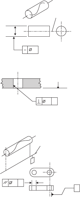
221 Basic mechanical design

Straightness

Squareness

A

Datum

Axis of hole to be within a cylindrical zone of diameter

0.1mm at 90°

Datum line

Parallelism

Axis is within a cylindrical

zone of diameter 0.1mm

0.1

A

B

Surface

to the datum surface A

0.1 A

0.1 B

Axis is within a cylindrical zone of diameter 0.1mm

parallel to the datum line A

Fig. 12.6 Straightness, parallelism and squareness

• Straightness: A hole or shaft can be straight

without being perpendicular to the surface

of the material.

• Parallelism: This is particularly relevant to

holes and is important when there is a

mating hole-to-shaft fit.

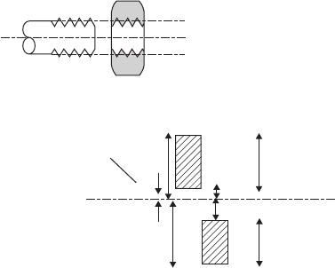
222 Aeronautical Engineer’s Data Book

• Squareness: The formal term for this is

perpendicularity. Simplistically, it refers to

the squareness of the axis of a hole to the

datum surface of the material through

which the hole is made.

12.4.3 Screw threads

There is a well-established system of toleranc-

ing adopted by ANSI/ASME, International

Standard Organizations and manufacturing

industry. This system uses the two complemen-

tary elements of fundamental deviation and

tolerance range to define fully the tolerance of

a single component. It can be applied easily to

components, such as screw threads, which join

or mate together (see Figure 12.7).

For screw threads, the tolerance layout shown

applies to major, pitch, and minor diameters

(although the actual diameters differ).

Fundamental

deviation (FD)

(end of range nearest

the basic size)

T

ES

ei

es

El

FD

NUT

'Zero line'

(basic size)

BOLT

Tolerance 'range'

FD is designated by a letter code, e.g. g,H

Tolerance range (T) is designated by a number code,

e.g. 5, 6, 7

Commonly used symbols are:

EI – lower deviation (nut)

ES – upper deviation (nut)

ei – lower deviation (bolt)

es – upper deviation (bolt)

Fig. 12.7 Tolerancing: screw threads

223 Basic mechanical design

• Fundamental deviation: (FD) is the distance

(or ‘deviation’) of the nearest ‘end’ of the

tolerance band from the nominal or ‘basic’

size of a dimension.

• Tolerance band: (or ‘range’) is the size of

the tolerance band, i.e. the difference

between the maximum and minimum

acceptable size of a toleranced dimension.

The size of the tolerance band, and the

location of the FD, governs the system of

limits and fits applied to mating parts.

Tolerance values have a key influence on the

costs of a manufactured item so their choice

must be seen in terms of economics as well as

engineering practicality. Mass-produced items

are competitive and price sensitive, and over-

tolerancing can affect the economics of a

product range.

12.5 Limits and fits

12.5.1 Principles

In machine element design there is a variety of

different ways in which a shaft and hole are

required to fit together. Elements such as

bearings, location pins, pegs, spindles and axles

are typical examples. The shaft may be required

to be a tight fit in the hole, or to be looser, giving

a clearance to allow easy removal or rotation.

The system designed to establish a series of

useful fits between shafts and holes is termed

limits and fits. This involves a series of tolerance

grades so that machine elements can be made

with the correct degree of accuracy and be inter-

changeable with others of the same tolerance

grade. The standards ANSI B4.1/B4.3 contain

the recommended tolerances for a wide range

of engineering requirements. Each fit is desig-

nated by a combination of letters and numbers

(see Tables 12.3, 12.4 and 12.5).

Figure 12.8 shows the principles of a

shaft/hole fit. The ‘zero line’ indicates the basic

or ‘nominal’ size of the hole and shaft (it is the

224 Aeronautical Engineer’s Data Book

Table 12.3 Classes of fit (imperial)

1. Loose running fit: Class RC8 and RC9. These are

used for loose ‘commercial-grade’ components where

a significant clearance is necessary.

2. Free running fit: Class RC7. Used for loose bearings

with large temperature variations.

3. Medium running fit: Class RC6 and RC5. Used for

bearings with high running speeds.

4. Close running fit: Class RC4. Used for medium-speed

journal bearings.

5. Precision running fit: Class RC3. Used for precision

and slow-speed journal bearings.

6. Sliding fit: Class RC2. A locational fit in which close-

fitting components slide together.

7. Close sliding fit: Class RC1. An accurate locational fit

in which close-fitting components slide together.

8. Light drive fit: Class FN1. A light push fit for long or

slender components.

9. Medium drive fit: Class FN2. A light shrink-fit

suitable for cast-iron components.

10. Heavy drive fit: Class FN3. A common shrink-fit for

steel sections.

11. Force fit: Class FN4 and FN5. Only suitable for high-

strength components.

Table 12.4 Force and shrink fits (imperial)

Nominal size Class

range, in

FN1 FN2 FN3 FN4 FN5

0.04–0.12 0.05 0.2 0.3 0.5

0.5 0.85 0.95 1.3

0.12–0.24 0.1 0.2 0.95 1.3

0.6 1.0 1.2 1.7

0.24–0.40 0.1 0.4 0.6 0.5

0.75 1.4 1.6 2.0

0.40–0.56 0.1 0.5 0.7 0.6

0.8 1.6 1.8 2.3

0.56–0.71 0.2 0.5 0.7 0.8

0.9 1.6 1.8 2.5

0.71–0.95 0.2 0.6 0.8 1.0

1.1 1.9 2.1 3.0

0.95–1.19 0.3 0.6 0.8 1.0 1.3

1.2 1.9 2.1 2.3 3.3

1.19–1.58 0.3 0.8 1.0 1.5 1.4

1.3 2.4 2.6 3.1 4.0

1.58–1.97 0.4 0.8 1.2 1.8 2.4

1.4 2.4 2.8 3.4 5.0

1.97–2.56 0.6 0.8 1.3 2.3 3.2

1.8 2.7 3.2 4.2 6.2

2.56–3.15 0.7 1.0

1.8 2.8 4.2

1.9 2.9 3.7 4.7 7.2

Limits in ‘mils’ (0.001 in).

225 Basic mechanical design

Upper deviation

(hole)

Shaft

Zero line

Basic size

Hole

Upper deviation

(shaft)

Lower deviation (shaft)

Lower deviation (hole)

Fig. 12.8 Principles of a shaft–hole fit

Table 12.5 Running and sliding fits (imperial)

Nominal Class

size

range, in RC1 RC2 RC3 RC4 RC5 RC6 RC7 RC8 RC9

0–0.12 0.1 0.1 0.3 0.3 0.6 0.6 1.0 2.5 4.0

0.45 0.55 0.95 1.3 1.6 2.2 2.6 5.1 8.1

0.12–0.24 1.5 0.15 0.4 0.4 0.8 0.8 1.2 2.8 4.5

0.5 0.65 1.2 1.6 2.0 2.7 3.1 5.8 9.0

0.24–0.40 0.2 0.2 0.5 0.5 1.0 1.0 1.6 3.0 5.0

0.6 0.85 1.5 2.0 2.5 3.3 3.9 6.6 10.7

0.40–0.71 0.25 0.25 0.6 0.6 1.2 1.2 2.0 3.5 6.0

0.75 0.95 1.7 2.3 2.9 3.8 4.6 7.9 12.8

0.71–1.19 0.3 0.3 0.8 0.8 1.6 1.6 2.5 4.5 7.0

0.95 1.2 2.1 2.8 3.6 4.8 5.7 10.0 15.5

1.19–1.97 0.4 0.4 1.0 1.0 2.0 2.0 3.0 5.0 8.0

1.1 1.4 2.6 3.6 4.6 6.1 7.1 11.5 18.0

1.97–3.15 0.4 0.4 1.2 1.2 2.5 2.5 4.0 6.0 9.0

1.2 1.6 3.1 4.2 5.5 7.3 8.8 13.5 20.5

3.15–4.73 0.5 0.5 1.4 1.4 3.0 3.0 5.0 7.0 10.0

1.5 2.0 3.7 5.0 6.6 8.7 10.7 15.5 24.0

Limits in ‘mils’ (0.001 in).

same for each) and the two shaded areas depict

the tolerance zones within which the hole and

shaft may vary. The hole is conventionally

shown above the zero line. The algebraic

difference between the basic size of a shaft or

hole and its actual size is known as the devia-

tion.

• It is the deviation that determines the

nature of the fit between a hole and a shaft.

226 Aeronautical Engineer’s Data Book

• If the deviation is small, the tolerance range

will be near the basic size, giving a tight fit.

• A large deviation gives a loose fit.

Various grades of deviation are designated by

letters, similar to the system of numbers used

for the tolerance ranges. Shaft deviations are

denoted by small letters and hole deviations by

capital letters. Most general engineering uses a

‘hole-based’ fit in which the larger part of the

available tolerance is allocated to the hole

(because it is more difficult to make an accurate

hole) and then the shaft is made to suit, to

achieve the desired fit.

Tables 12.4 and 12.5 show suggested clear-

ance and fit dimensions for various diameters

(ref.: ANSI B4.1 and 4.3).

Table 12.6 Metric fit classes

1. Easy running fit: H11-c11, H9-d10, H9-e9. These are

used for bearings where a significant clearance is

necessary.

2. Close running fit: H8-f7, H8-g6. This only allows a

small clearance, suitable for sliding spigot fits and

infrequently used journal bearings. This fit is not

suitable for continuously rotating bearings.

3. Sliding fit: H7-h6. Normally used as a locational fit in

which close-fitting items slide together. It incorporates

a very small clearance and can still be freely

assembled and disassembled.

4. Push fit: H7-k6. This is a transition fit, mid-way

between fits that have a guaranteed clearance and

those where there is metal interference. It is used

where accurate location is required, e.g. dowel and

bearing inner-race fixings.

5. Drive fit: H7-n6. This is a tighter grade of transition fit

than the H7–k6. It gives a tight assembly fit where the

hole and shaft may need to be pressed together.

6. Light press fit: H7-p6. This is used where a hole and

shaft need permanent, accurate assembly. The parts

need pressing together but the fit is not so tight that it

will overstress the hole bore.

7. Press fit: H7-s6. This is the tightest practical fit for

machine elements such as bearing bushes. Larger

interference fits are possible but are only suitable for

large heavy engineering components.

227 Basic mechanical design

12.5.2 Metric equivalents

The metric system (ref. ISO Standard EN

20286) ISO ‘limits and fits’ uses seven popular

combinations with similar definitions (see

Table 12.6 and Figure 12.9).

Clearance fits

Easy running Close

running

Sliding Push Drive Light

press

Press

TolsTolsTolsTolsTolsTolsTolsTolsTols

H11

-80

-170

-95

-205

-110

-240

-120

-280

-130

-290

+36

0

+43

0

+52

0

+62

0

-40

-98

-50

-120

-69

-149

-80

-180

+36

0

+43

0

+52

0

+62

0

-25

-61

-32

-75

-40

-92

-50

-112

+22

0

+27

0

+33

0

+39

0

-12

-28

-16

-34

-20

-41

-25

-50

+15

0

+18

0

+21

0

+25

-50

-5

-14

-6

-17

-7

-20

-9

-25

+15

0

+18

0

+21

0

+25

0

-9

0

-11

0

-13

0

-16

0

+15

0

+18

0

+21

0

+25

0

+10

+1

+12

+1

+15

+2

+18

+2

+15

0

+18

0

+21

0

+25

0

+19

+10

+23

+12

+28

+15

+33

+17

+15

0

+18

0

+21

0

+25

0

+24

+15

+29

+18

+35

+22

+42

+26

+15

0

+18

0

+21

0

+25

0

+32

+23

+39

+28

+48

+35

+59

+43

+90

0

+110

0

+130

0

+140

0

+160

0

H9 H8 f7 H7 g6 H7 H7 H7k6 n6 H7 p6 H7 s6h6e9d10

Nominal

size

in mm

6-10

10-18

18-30

30-40

40-50

Holes

Shafts

H11

H9 H9

H8

H7

c11

d10

e9

f7

g6 h6

H7 H7

k6

p5 p6

s6

fits fits

Tols*

c11 H9

H7 H7

Transmission Interference

*Tolerance units in 0.001 mm Data from BS 4500

Fig. 12.9 Metric fits

12.6 Surface finish

Surface finish, more correctly termed ‘surface

texture’, is important for all machine elements

that are produced by machining processes such

as turning, grinding, shaping, or honing. This

applies to surfaces which are flat or cylindrical.

Surface texture is covered by its own technical

standard: ASME/ANSI B46.1: 1995: Surface

Texture. It is measured using the parameter R

a

which is a measurement of the average distance

between the median line of the surface profile

and its peaks and troughs, measured in

microinches (µ in). There is another system

from a comparable European standard, DIN

ISO 1302, which uses a system of N-numbers –

228 Aeronautical Engineer’s Data Book

it is simply a different way of describing the

same thing.

12.6.1 Choice of surface finish: approximations

Basic surface finish designations are:

• Rough turned, with visible tool marks:

500 µin R

a

(12.5 µm or N10)

• Smooth machined surface:

125 µin R

a

(3.2 µm or N8)

• Static mating surfaces (or datums):

63 µin R

a

(1.6 µm or N7)

• Bearing surfaces:

32 µin R

a

(0.8 µm or N6)

• Fine ‘lapped’ surfaces:

1 µin R

a

(0.025 µm or N1)

Figure 12.10 shows comparison between the

different methods of measurement.

Finer finishes can be produced but are more

suited for precision application such as instru-

ments. It is good practice to specify the surface

finish of close-fitting surfaces of machine

elements, as well as other ASME/ANSI Y

14.5.1 parameters such as squareness and paral-

lelism.

Fine finish Rough finish

R

, (µm) 0.025 0.05 0.1 0.2 0.4 0.8 1.6 3.2 6.3 12.5 25 50

BS1134

R

, (µinch)

1 2 4 8 16 32 63 125 250 500 1000 2000

ANSI B46.1

N

-grade

N1 N2 N3 N4 N5 N6 N7 N8 N9 N10 N11 N12

DIN ISO 1302

Ground finishes Smooth Medium

turned turned

Seal-faces and Rough turned finish

running surfaces

A prescribed surface finish is shown on a drawing as

– on a metric drawing this means 1.6µm

R

a

16

Fig. 12.10 Surface measurement

229 Basic mechanical design

12.7 Computer aided engineering

Computer Aided Engineering (CAE) is the

generic name given to a collection of computer

aided techniques used in aeronautical and

other types of mechanical engineering.

Computer Aided Engineering (CAE)

comprises:

• CAD: Computer Aided Design (or Drafting)

– Computer aided design is the application

of computers to the conceptual/design

part of the engineering process. It

includes analysis and simulation.

– Computer aided drafting is the application

of computer technology to the production

of engineering drawings and images.

• CAM: Computer Aided Manufacture

relates to the manufacture of a product

using computer-controlled machine tools of

some sort.

• MRP: Materials Requirements Planning/

Manufacturing Resource Planning: defines

when a product is made, and how this fits in

with the other manufacturing schedules in

the factory.

• CIM: Computer Integrated Manufacture is

the integration of all the computer-based

techniques used in the design and manufac-

ture of engineering products.

Figure 12.11 shows a general representation of

how these techniques fit together.

12.7.1 CAD software

CAD software exists at several levels within an

overall CAE system. It has different sources,

architecture and problems. A typical structure is:

• Level A: Operating systems: Some are

manufacturer-specific and tailored for use

on their own systems.

• Level B: Graphics software: This governs

the type and complexity of the graphics that

both the CAD and CAM elements of a

CAE system can display.

230 Aeronautical Engineer’s Data Book

CAE

CAD CAM

100110010

100101001

010101010

Central CAD/CAM

computer facility

Analysis and

modelling

Numerical

control

Process

planning

Drafting

Factory

Testing

management

Fig. 12.11 CAE, CAD and CAM

• Level C: Interface/Exchange software: This

comprises the common software that will be

used by all the CAD/CAM application, e.g.

user interface, data exchange etc.

• Level D: Geometric modelling programs:

Most of these are designed to generate an

output which can be translated into geomet-

ric form to guide a machine tool.

• Level E: Applications software: This is the

top level of vendor-supplied software and

includes drafting, and analysis/simulation

facilities.

• Level F: User-defined software: Many

systems need to be tailored before they can

become truly user-specific. This category

231 Basic mechanical design

contains all the changes required to adapt

vendor software for custom use.

12.7.2 Types of modelling

CAD software packages are divided into those

that portray two-dimensional or three-dimen-

sional objects. 3D packages all contain the

concept of an underlying model. There are

three basic types as shown in Figure 12.12

Wireframe models

Although visually correct these do not contain

a full description of the object. They contain no

information about the surfaces and cannot

differentiate between the inside and outside.

They cannot be used to link to a CAM system.

Surface models

Surface models are created (conceptually) by

stretching a two-dimensional ‘skin’ over the

Wireframe model

between inside and

It is possible to get

No differentiation

meaningless

‘

nonsense’ models

outside

like this

S

urface model

All surfaces and their

boundaries are defined

Although the model

and recognized by the

appears

solid, there

model

is no recognition of

what lies inside the

sur

faces

Solid model

The model is

recognized as a

solid object

Various techniques of solid

modelling include:

• BR (Boundary

Representation)

• CSG (Constructive Solid

Geometr

y)

• FM (Faceted Modelling)

Fig. 12.12 Types of modelling

232 Aeronautical Engineer’s Data Book

edges of a wireframe to define the surfaces.

They can therefore define structure bound-

aries, but cannot distinguish a hollow object

from a solid one. Surface models can be used

for geometric assembly models etc., but not

analyses which require the recognition of the

solid properties of a body (finite element stress

analysis, heat transfer etc.).

Solid models

Solid models provide a full three-dimensional

geometrical definition of a solid body. They

require large amounts of computer memory for

definition and manipulation but can be used for

finite element applications. Most solid model-

ling systems work by assembling a small

number of ‘building block’ reference shapes.

12.7.3 Finite Element (FE) analysis

FE software is the most widely used type of

engineering analysis package. The basic idea is

that large three-dimensional areas are subdi-

vided into small triangular or quadrilateral

(planar) or hexahedral (three-dimensional)

elements then subject a to solution of multiple

simultaneous equations. The general process is

loosely termed mesh generation. There are four

types which fall into the basic category.

• Boundary Element Modelling (BEM): This

is a simplified technique used for linear or

static analyses where boundary conditions

(often assumed to be at infinity) can be

easily set. It is useful for analysis of cracked

materials and structures.

• Finite Element Modelling (FEM): The

technique involves a large number of

broadly defined (often symmetrical)

elements set between known boundary

conditions. It requires large amounts of

computing power.

• Adaptive Finite Element Modelling

(AFEM): This is a refinement of FEM in

which the element ‘mesh’ is more closely

233 Basic mechanical design

defined in critical areas. It produces better

accuracy.

• Finite Difference Method: A traditional

method which has now been superseded by

other techniques. It is still used in some

specialized areas of simulation in fluid

mechanics.

12.7.4 Useful references

Standards: Limits, tolerances and surface

texture

1. ANSI Z17.1: 1976: Preferred numbers

.

2. ANSI B4.2: 1999: Preferred metric limits and

fits

.

3. ANSI B4.3: 1999: General tolerances for

metric dimensioned products

.

4. ANSI/ASME Y14.5.1 M: 1999: Dimension-

ing and Tolerances – mathematical defini-

tions of principles.

5. ASME B4.1: 1999: Preferred limits and fits

for cylindrical parts

.

6. ASME B46.1: 1995: Surface texture (surface

roughness, waviness and lay)

7. ISO 286–1: 1988: ISO system of limits and fits.

Standards: Screw threads

1. ASME B1.1: 1989: Unified inch screw

threads (UN and UNR forms)

.

2. ASME B1.2: 1991: Gauges and gauging for

unified screw threads

.

3. ASME B1.3M: 1992: Screw thread gauging

systems for dimensional acceptability – inch

and metric screws

.

4. ASME B1.13: 1995: Metric screw threads

.

5. ISO 5864: 1993: ISO inch screw threads –

allowances and tolerances.

Websites

1. For a general introduction to types of

CAD/CAM go to ‘The Engineering Zone’ at

www.flinthills.com/~ramsdale/EngZone/cad

cam.htm. This site also contains lists of links

to popular journal sites such as

CAD/CAM

magazine and CAE magazine.

234 Aeronautical Engineer’s Data Book

2. ‘Finite Element Analysis World’ includes

listings of commercial software. Go to:

www.comco.com/feaworld/feaworld.html.

3. For a general introduction to Computer

Integrated Manufacture (CIM) go to:

www.flinthills.com/~ramsdale/EngZone/

cim.htm.

4. The International Journal of CIM, go to:

www.tandfdc.com/jnls/cim.htm.

5. For an online introductory course on CIM,

go to: www.management.mcgill.ca/course/

msom/MBA/mgmt-tec/students/cim/TEST.

htm.

6. For a list of PDM links, go to: www.

flinthills.com/~ramsdale/EngZone/pdm.htm.

7. The PDM Information Center PDMIC is a

good starting point for all PDM topics. Go

to: www.pdmic.com/. For a bibliography

listing, go to: www.pdmic.com/bilbliogra-

phies/index.html.

Section 13

Reference sources

13.1 Websites

Table 13.1 provides a list of useful aeronautical

websites.

13.2 Fluid mechanics and aerodynamics

Flight Dynamic Principles. M.V. Cook. ISBN 0-

340-63200-3. Arnold 1997.

Performance and Stability of Aircraft. J.B.

Russell. ISBN 0-340-63170-8. Arnold 1996.

Aerodynamics for Engineering Students

, 4th ed.

E.L. Houghton, P.W. Carpenter. ISBN 0-

340-54847-9. Arnold 1993.

Introduction to Fluid Mechanics

. Y. Nakayama,

R.F. Boucher. ISBN 0-340-67649-3. Arnold

1999.

Fluid Mechanics: An Interactive Text. J.A.

Liggett, D.A. Caughey. ISBN 0-7844-0310-4.

AIAA: 1998. This is a multimedia CD-ROM

for fluid mechanics.

13.3 Manufacturing/materials/structures

Composite Airframe Structures, Michael C.Y.

Niu, Conmilit Press Ltd, Hong Kong, 1992.

D.H. Middleton, ‘The first fifty years of

composite materials in aircraft construction’,

Aeronautical Journal

, March 1992, pp. 96–104

Aerospace Thermal Structures and Materials for

a New Era

. ISBN 1-56347-182-5. AIAA

publication 1995.

Aircraft Structures for Engineering Students,

3rd ed. T.H.G. Megson. ISBN 0-340-70588-4.

Arnold 1999.

236

Table 13.1 Useful aeronautical websites

Advisory Group for Aerospace Research and Development (AGARD)

Aerospace Engineering Test Establishment (AETE)

Aerospace Technical Services (Australia)

Aerospatiale

Air Force Development Test Center (AFDTC)

Air Force Flight Test Center (AFFTC)

Air Force Operational Test and Evaluation Center (AFOTEC)

Airbus Industrie

Aircraft Data

Aircraft Locator – Manufacturer Index

Airports Council International (ACI)

Allied Signal

American and Canadian Aviation Directory

American Institute of Aeronautics and Astronautics (AIAA)

American Society of Mechanical Engineering

Army Aviation Technical Test Center (ATTC)

Arnold Engineering Development Center (AEDC)

Australian Centre for Test and Evaluation

http://www.wkap.nl/natopco/pco_aga.htm

http://www.achq.dnd.ca/aete/index.htm

http://www.aerospace.com.au/

http://www.aerospatiale.fr/

http://www.eglin.af.mil/afdtc/afdtc.html

http://www.edwards.af.mil/

http//www.afotec.af.mil/

http://www.airbus.com/

http://www.arnoldpublishers.com/aerodata/appendices/data

-a/default.htm

http://www.brooklyn

cuny.edu/rec/air/museums/manufact/manufact.html

http://www.airports.org/

http://www.alliedsignal.com/

http://hitech.superlink/net/av/

http://www.aiaa.org/

http://www.asme.org/

http://www.attc.army.mil/

http://info.arnold.af.mil/

http://www.acte.unisa.edu.au/weblinks.htm

237

BOEING Technology Services

British Aerospace

CASA

Civil Aviation Authority (CAA)

Daimler Chrysler Aerospace

Defence Evaluation & Research Agency (DERA) United Kingdom

Defence Technical Information Center (DTIC)

DefenseLINK

Director, Test, Systems Engineering and Evaluation (DTSE&E)

Directory of Technical Engineering and Science Societies and Organizations

DLR – German Aerospace Research Establishment

DoD-TECNET: The Test and Evaluation Community Network

Dryden Flight Research Center (DFRC) – NASA

Edinburgh Engineering Virtual Library (EEVL)

Electronic Systems Center (ESC)

Engine Data

Experimental Aircraft Association (EAA)

Federal Aviation Administration

National Aeronautical and Space Administration (NASA)

Flight Test Safety Committee (FTSC)

Fokker

http://www.boeing.com/bts/

http://www.bae.co.uk/

http://www.casa.es/

http://www.caa.co.uk/

http://www.dasa.com/

http://www.dera.gov.uk/

http://www.dtic.dla.mil/

http://www.dtic.dla.mil/defenselink/index.html

http://www.acq.osd.mil/te/index.html

http://www.techexpo.com/tech_soc.html

http://www.dlr.de/

http://www.tecnet0.jcte.jcs.mil:9000/index.html

http://www.dfrc.nasa.gov/

http://www.eevl.ac.uk/

http://www.hanscom.af.mil/

http://www.arnoldpublishers.com/aerodata/appendices/data

-b/default.htm

http://www.eaa.org/

http//www.faa.gov/

http://www.nasa.gov/

http://www.netport.com/setp/ftsc/index.html

http://www.fokker.com/

238

Table 13.1 Continued

General Electric Aircraft Engines

Institution of Electrical and Electronic Engineers (IEEE)

Institution of Mechanical Engineers (IMechE)

International Federation of Airworthiness

International Test and Evaluation Association (ITEA)

International Test Pilots School (ITPS), United Kingdom

Major Range Test Facilities Base (MRTFB)

McDonnell Douglas Corporation

National Aerospace Laboratory (Netherlands)

National Test Pilot School (NTPS)

Naval Air Warfare Center – Aircraft Division (NAWCAD)

Naval Air Warfare Center – US Navy Flight Test

Naval Air Warfare Center – Weapons Division (NAWCWPNS)

Nellis Air Force Base

North Atlantic Treaty Organization (NATO)

Office National d’Études et de Recherches Aérospatiales (France)

Office of the Director; Operational Test & Evaluation

Pratt & Witney

Rolls-Royce

Royal Aeronautical Society

http://www.ge.com/aircraftengines/

http://www.ieee.org/

http://www.imeche.org.uk

http://www.ifairworthy.org/

http://www.itea.org/

http://www.itps.uk.com/

http://www.acq.osd.mil/te/mrtfb.html

http//www.mdc.com/

http://www.nlr.nl/

http://www.ntps.com/

http://www.nawcad.navy.mil/

http://www.flighttest.navair.navy.mil/

http://www.nawcwpns.namy.mil/

http://www.nellis.af.mil/

http://www.nato.int/

http://www.onera.fr/

http://www.dote.osd.mil/

http://www.pratt-whitney.com/

http://www.rolls-royce.co.uk/

http://www.raes.org.uk/default.htm

239

Society of Automotive Engineers (SAE)

Society of Experimental Test Pilots (SETP)

Society of Flight Test Engineers (SFTE), North Texas Chapter

United States Air Force Museum

University Consortium for Continuing Education (UCCE)

University of Tennessee Space Institute, Aviation Systems Department

Virginia Tech Aircraft Design Information Sources

VZLYOT Incorporated (Russia)

http://www.sae.org/

http://www.netport.com/setp/

http://www.rampages.onramp.net/~sfte/

http://www.wpafb.af.mil/museum/index.htm

http://www.ucce.edu/

http://www.utsi.edu/Academic/graduate.html

http://www.aoe.vt.edu/Mason/ACinfoTOC.html

http://www.dsuper.net/~vzlyot/

Edinburgh (UK) Engineering Virtual Library (EEVL)

EEVL is one of the best ‘gateway’ sites to quality aeronautical engineering information on the internet. It contains:

The EEVL catalogue: Descriptions and links to more than 600 aeronautical and 4500 engineering-related websites which can be

browsed by engineering subject or resource type (journals, companies, institutions etc.).

Engineering newsgroups: Access to over 100 engineering newsgroups.

Top 25 and 250 sites: Records of the most visited engineering websites.

Access the EEVL site at http:/www.eevl.ac.uk

240 Aeronautical Engineer’s Data Book

13.4 Aircraft sizing/multidisciplinary design

C. Bil, ‘ADAS: A Design System for Aircraft

Configuration Development’, AIAA Paper

No. 89-2131. July 1989.

S. Jayaram, A. Myklebust and P. Gelhausen,

‘ACSYNT – A Standards-Based System for

Parametric Computer Aided Conceptual

Design of Aircraft’, AIAA Paper 92-1268,

Feb. 1992.

Ilan Kroo, Steve Altus, Robert Braun, Peter

Gage and Ian Sobieski, ‘Multidisciplinary

Optimization Methods for Aircraft Prelimi-

nary Design’, AIAA Paper 94-4325, 1994.

P.J. Martens, ‘Airplane Sizing Using Implicit

Mission Analysis’, AIAA Paper 94-4406,

Panama City Beach, Fl., September 1994.

Jane Dudley, Ximing Huang, Pete MacMillin,

B. Grossman, R.T. Haftka and W.H. Mason,

‘Multidisciplinary Optimization of the High-

Speed Civil Transport’, AIAA Paper

95–0124, January 1995.

The anatomy of the airplane, 2nd ed. D. Stinton.

ISBN 1-56347-286-4. Blackwell, UK: 1998.

Civil jet aircraft design. L.R. Jenkinson, P.

Simpkin and D. Rhodes. ISBN 0-340-74152.

Arnold 1999.

13.5 Helicopter technology

Basic Helicopter Aerodynamics. J. Seddon.

ISBN 0-930403-67-3. Blackwell UK: 1990.

The Foundations of Helicopter Flight. S.

Newman. ISBN 0-340-58702-4. Arnold 1994.

13.6 Flying wings

The Flying Wings of Jack Northop. Gary R.

Pape with Jon M. Campbell and Donna

Campbell, Shiffer Military/Aviation History,

Atglen, PA, 1994.

Tailless Aircraft in Theory and Practice. Karl

Nickel and Michael Wohfahrt, AIAA,

Washington, 1994.

241 Reference sources

David Baker, ‘Northrop’s big wing – the B-2’

Air International, Part 1, Vol. 44, No. 6, June

1993, pp. 287–294.

Northrop B-2 Stealth Bomber. Bill Sweetman.

Motorbooks Int’l. Osceola, WI, 1992.

13.7 Noise

Aircraft Noise. Michael J. T. Smith, Cambridge

University Press, Cambridge, 1989.

E.E. Olson, ‘Advanced Takeoff Procedures for

High-Speed Civil Transport Community

Noise Reduction’, SAE Paper 921939, Oct.

1992.

13.8 Landing gear

Chai S. and Mason W.H. ‘Landing Gear

Integration in Aircraft Conceptual Design,’

AIAA Paper 96–4038, Proceedings of the 6th

AIAA/NASA/ISSMO Symposium on Multi-

disciplinary Analysis and Optimization, Sept.

1996. pp. 525–540. Acrobat format.

S.J. Greenbank, ‘Landing Gear – The Aircraft

Requirement’, Proceedings of Institution of

Mechanical Engineers

(UK), Vol. 205, 1991,

pp.27–34.

Airframe Structural Design. M.C.Y. Niu.

Conmilit Press, Ltd, Hong Kong, 1988. This

book contains a good chapter on landing

gear design.

S.F.N. Jenkins. ‘Landing Gear Design and

Development’, Institution of Mechanical

Engineers (UK), proceedings, part G1,

Journal of Aerospace Engineering

, Vol. 203,

1989.

13.9 Aircraft operations

Aircraft Data for Pavement Design. American

Concrete Pavement Association, 1993.

Airport Engineering, 3rd ed. Norman Ashford

and Paul H. Wright. John Wiley & Sons, Inc.,

1992.

242 Aeronautical Engineer’s Data Book

13.10 Propulsion

Walter C. Swan and Armand Sigalla, ‘The

Problem of Insalling a Modern High Bypass

Engine on a Twin Jet Transport Aircraft’, in

Aerodynamic Drag, AGARD CP-124, April

1973.

The Development of Piston Aero Engines. Bill

Gunston. Patrick Stephens Limited, UK,

1993.

Aircraft Engine Design. J.D. Maltingly, W.H.

Heiser, D.H. Daley. ISBN 0-930403-23-1.

AIAA Education Series, 1987.

X

Appendix 1:

Aerodynamic stability and

control derivatives

Table A1.1 Longitudinal aerodynamic stability derivatives

Dimensionless Multiplier Dimensional

˚

X

u



2

1



X

M



V

0

S

˚

X

w

X

w



2

1



X

w



V

0

S

=



2

1



X

w˚



Sc

˚

X

q

=



2

1





V

0

Sc

q

˚

Z

u



2

1



Z

M



V

0

S

˚

Z

w

Z

w



2

1



Z

w



V

0

S

=



2

1



˚

Z

w



Sc

˚

Z

q

=



2

1



Z



V

0

Sc

q

˚

M

u

=



2

1



M



V

0

Sc

u

˚

M

w

M

w

=



2

1



M

w



V

0

Sc

=

2



2

1



˚

M

w



Sc

˚

M

q

=

2



2

1



M



V

0

Sc

q

Table A1.2 Longitudinal control derivatives

Dimensionless Multiplier Dimensional

X



Z



M



X



Z



M



2

S

1



2



V

0

2

S

1



2



V

0

2

Sc

=

1



2



V

0

1

=

c



X

˚



Z

˚



M

˚



X

˚



Z

˚



M

˚



244 Aeronautical Engineer’s Data Book

Table A1.3 Lateral aerodynamic stability derivatives

Dimensionless Multiplier Dimensional

Y



1



2



V

0

S Y

˚



Y

p

r

1



2

1



2



V

0

Sb



V

0

Sb

Y

˚

p

Y

˚

r

L



1



2



V

0

Sb L

˚



L

p

L

r



V

0

Sb

2

1



2

1



2



V

0

Sb

2

L

˚

p

L

˚

r

N



1



2



V

0

Sb N

˚



N

p

r

N



V

0

Sb

2

1



2

1



2



V

0

Sb

2

N

˚

p

N

˚

r

Table A.14 Lateral aerodynamic control derivatives

Dimensionless Multiplier Dimensional

Y



L



N



Y



L



N



2

S

1



2



V

0

2

Sb

1



2



V

0

2

Sb

1



2



V

0

2

S

1



2



V

0

2

Sb

1



2



V

0

2

Sb

1



2



V

0

Y

˚



L

˚



N

˚



Y

˚



L

˚



N

˚



Appendix 2:

Aircraft response transfer

functions

Table A2.1 Longitudinal response transfer functions



is elevator input.

Common denominator polynomial ∆(s) = as

4

+ bs

3

+ cs

2

+

ds + e

a mI

y

(m – Z

˚

)

w

b I

y

(X

˚

u

Z

˚

w˚

– X

˚

w˚

Z

˚

u

) – mI

Y

(X

˚

+ Z

˚

w

) – mM

w˚

(Z

˚

q

+

u

˚

mU

e

) – mM

q

(m – Z

˚

)

w

˚

c I

y

(X

˚

u

Z

˚

w˚

– X

˚

w

Z

˚

u

) + (X

˚

M

˚

– X

˚

M

˚

u

)(Z

˚

q

+ mU

e

)

˚ ˚

u w w

+ Z

˚

u

(X

˚

w˚

M

q

– X

˚

M

˚

) + (X

˚

M

˚

– X

˚

M

˚

u

)(m – Z

˚

)

˚ ˚

q w u q q w

+ m(M

˚

q

Z

˚

w

– M

˚

w

Z

˚

q

) + mW

e

(M

w˚

Z

˚

u

– M

u

Z

˚

w˚

)

+ m

2

(M

˚

g sin



– u

e

M

˚

w

)

˚

w e

d (X

˚

u

M

w

– X

˚

w

M

˚

u

)(Z

˚

q

+ mU

e

)

˚ ˚

+ (M

u

Z

˚

w

– M

w

Z

˚

u

)(X

˚

q

mW

e

) + M

˚

q

(X

˚

w

Z

˚

u

– X

˚

u

Z

˚

w

)

+ mg cos



e

(M

˚

w˚

Z

˚

u

+ M

˚

u

(m – Z

˚

)) + mg sin



e

(X

˚

w˚

M

˚

uw

– X

˚

u

M

˚

w

+ mM

˚

w

)

˚ ˚

+ mg sin



(X

˚

w

M

˚

u

– X

˚

u

M

w

) + mg cos



(M

w

Z

˚

u

–

e e

M

˚

u

Z

˚

w

)

˚

e mg sin



(X

˚

w

M

˚

u

– X

˚

u

M

˚

w

) + mg cos



(M

w

Z

˚

u

–

e e

M

˚

u

Z

˚

w

)

Numerator polynomial N



3

(s) = as

2

+ bs

2

+ cs + d

a I

y

(X

˚

Z

˚



+ X

˚



(m – Z

˚

))

w w

b X

˚



(–I

y

Z

˚

w

+ mU

e

) – M

˚

q

(m – Z

˚

))

w

˚

+ Z

˚



(I

y

X

˚

w

– X

˚

w˚

M

q

+ M

˚

(X

˚

q

– mW

e

))

w

+ M

˚



((X

˚

q

– mW

e

)(m – Z

˚

) + X

˚

w˚

(Z

˚

q

+ mU

e

))

˚ ˚

w

c X

˚



(Z

˚

w

M

˚

q

– (M

w

(Z

˚

q

+ mU

e

) + mg sin



e

M

w˚

)

˚

+ Z

˚



(M

˚

w

(X

˚

q

– mW

e

) – X

˚

M

q

– mg cos



e

M

˚

w˚

)

w

+ M

˚



(X

˚

w

(Z

˚

q

+ mU

e

) – Z

˚

w

(X

˚

q

– mW

e

) – mg cos



(m

e

– Z

˚

) – mg sin



e

X

˚

w˚

)

˚

w



d X

˚



M

˚

w

mg sin



– Z

˚



M mg cos



+ M

˚



(Z

˚

mg cos

e

– X

˚

w

mg sin



e

)

e w e w

246 Aeronautical Engineer’s Data Book

Table A2.2 Lateral-directional response transfer functions

in terms of dimensional derivatives

 is aileron input

Demoninator polynomial ∆(s) = s(as

4

+ bs

3

+ cs

2

+ ds + e)

a m

(I

x

I

z

– I

2

xz

)

b –Y

˚

v

(I

x

I

z

– I

2

xz

) – m(I

x

N

˚

r

+ I

xz

L

˚

r

) – m(I

z

L

˚

p

+ I

xz

N

˚

p

)

c Y

˚

v

(I

x

N

˚

r

+ I

xz

L

˚

r

) + Y

˚

(I L

˚

p

+ I

xz

N

˚

p

) – (Y

˚

+ mW

e

)(I

v z p z

L

˚

v

+ I

xz

N

˚

v

)

– (Y

˚

– mU

e

)(I

x

N

˚

v

+ I

xz

L

˚

v

) + m(L

˚

p

N

˚

r

– L

˚

r

N

˚

p

)

r

d – (Y

˚

(L

˚

N

˚

– L

˚

p

N

˚

r

) + (Y

˚

p

+ mW

e

)(L

˚

v

N

˚

r

– L

˚

r

N

˚

v

)

v r p

(Y

˚

– mU

e

)(L

˚

p

N

˚

v

– L

˚

v

N

˚

p

)

r

– mg cos



e

(I

z

L

˚

v

+ I

xz

N

˚

v

) – mg sin



e

(I

x

N

˚

v

+ I

xz

L

˚

v

)

e mg cos



e

(L

˚

v

N

˚

r

– L

˚

r

N

˚

v

) + mg sin



e

(L

˚

p

N

˚

v

– L

˚

v

N

˚

p

)

Numerator polynomial N

v



(s) = s(as

3

+ bs

2

+ cs + d)

a Y

˚



(I

x

I

z

– I

2

xz

)

b Y

˚



(–I

x

N

˚

r

– I

z

L

˚

p

– I

xz

(L

˚

r

N

˚

p

)) + L

˚



(I

z

(Y

˚

+ mW

e

) +

I

xz

(Y

˚

r

– mU

e

))

p

+ N

˚



(I

x

(Y

˚

– mU

e

) + I

xz

(Y

˚

p

+ mW

e

))

c Y

˚



(L

˚

p

N

˚

r

– L

˚

r

N

˚

p

)

r

I

+ L

˚



(N

˚

p

(Y

˚

– mU

e

) – N

˚

(Y

˚

p

+ mW

e

) + mg(I

z

cos



+

xz

sin



e

))

r r e

+ N

˚



(L

˚

r

(Y

˚

p

– mW

e

) – L

˚

p

(Y

˚

+ mU

e

) + mg(I sin



e

+

I

xz

cos



e

))

r x

d L

˚



(N

˚

p

mg sin



– N

˚

r

mg cos



e

) + N

˚



(L

˚

mg cos



– L

˚

p

mg cos



e

)

e r e

Appendix 3:

Approximate expressions for the

dimensionless aerodynamic

stability and control derivatives



















248

Table A3.1 Longitudinal aerodynamic stability derivatives

Small perturbation derivatives referred to aircraft wind axes

Derivative Description Expression Comments

C

X

u

Axial force due to velocity – 2C

D

– V

0

V

D



∂



∂ V

∂



∂

1

Drag and thrust effects due to velocity

perturbation

+



V

0

S



2

1



C

D





∂



∂

Lift and drag effects due to incidence

perturbation

X

w

Axial force due to incidence C

L

–

C

D˚

r˚



∂



∂

Tailplane drag effect, usually negligible

Axial force due to pitch rate – V

X

q



r

T

Tailplane drag due to downwash lag effect

(added mass effect)

C

D

– V



r

∂

T

˚r˚



∂





d



d

q

d



d

 XX

w

Axial force due to downwash lag

˚

Z

u

Normal force due to velocity – 2C

L

– V

0

C

V

C

L



∂



∂

L



∂



∂

Lift effects due to velocity perturbation

Lift and drag effects due to incidence

perturbation

Z

w

Normal force due to ‘incidence’ – C

D

–































249



r



1

Tailplane lift effect

Z Normal force due to pitch rate – V

q

Tailplane lift due to downwash lag effect

(added mass effect)

d d

= Z

d d

Z

w

Normal force due to downwash lag – V

˚



r



1 q

C

M

u

Pitching moment due to velocity V

0

V

m



∂



∂

Mach dependent, small at low speed

C

= –K

n

d

m





d

Pitch stiffness, dependent on static margin

M

w

Pitching moment due to ‘incidence’

– V



T

=

c

l

T



=

c

l

T



Pitch damping, due mainly to tailplane

 ZM Pitching moment due to pitch rate

q q

d

M

w

Pitching moment due to downwash lag

˚

–V



T



1

=

c

l

T



 M

d

q

d

Pitch damping, due to downwash lag effect at

tailplane

Table A3.2 Small perturbation derivatives referred to aircraft wind axes

Derivative Description Expression Comments

Y

v

Sideforce due to

sideslip





S

B



y

B

–



S

F





1

F



Always negative and hence

stabilizing

L

v

Rolling moment

due to sideslip

(i) wing with dihedral –



S

1

s





s

0

c

y

a

y

ydy Lateral static stability, determined by

total dihedral effect. Most accessible

(ii) wing with aft sweep –



2C

L

t

S

a

s

n 

1

/

4





s

0

c

y

ydy

approximate contribution is given

(iii) fin contribution a

1

F

V



F



h

l

F



N

v

Yawing moment

due to sideslip

(i) fin contribution a

1

F

V



F

Natural weathercock stability,

dominated by fin effect

Y

p

Sideforce due to

roll rate

(i) fin contribution –



S

1

b





H

F

0

a

h

c

h

hdh Fin effect dominates, often negligible

250



 



251

L



s

(a

2Ss



2

1

Rolling moment

p

due to roll rate

2

dy

Roll damping wing effects dominate

but fin and tailplane contribute

(i) wing contribution + C

D

)c

y

–

y

0



s

2Ss



2

1 dC

N Yawing moment

p

due to roll rate

D



da

2

dy(i) wing contribution C

L

– – c

y

0

y



F

a

1

F

Many contributions, but often

Y

r

Sideforce due to

(i) fin contribution V

yaw rate negligible



s

C

L

Ss



2

1

L

r

Rolling moment

due to yaw rate

2

dy(i) wing contribution c

y

0

h

V



F



b

l

 – L

v(fin)

b

F



(ii) fin contribution a

1

F



s

C

D

N

r

Yawing moment Yaw damping, for large aspect ratio

2

dy(i) wing contribution c

y

1

Ss



2

due to yaw rate

0

y

rectangular wing, wing contribution is

approximately C

D

/

6

l l

VV



F



b

 –

F



b

(ii) fin contribution

N

v(fin)

a

1

F

252 Aeronautical Engineer’s Data Book

Table A3.3 Longitudinal aerodynamic control derivatives

Small perturbation derivatives referred to aircraft wind axes

Derivative Description Expression Comments

X



Axial force

due to

elevator

– 2



S

T



k

T

C

L

T

a

2

Usually

insignificantly

small

Z



Normal

force due

to elevator

–



S

T



a

2

M



Pitching – V



T

a

2

Principal

moment measure of

due to pitch control

elevator power

Appendix 4:

Compressible flow tables

Table A4.1 Subsonic flow (isentropic flow,



= 7/5)

Notation:

M = Local flow Mach number

P/P = Ratio of static pressure to total pressure

o



/



= Ratio of local flow density to stagnation density

o

T/T

o

= Ratio of static temperature to total temperature



= (1 – M

2

) = Compressibility factor

V/a* = Local velocity/speed of sound at sonic point

q/P = Dynamic pressure/total pressure

o

A/A* = Local flow area/flow area at sonic point

M P/P

o

/

o

T/T

o

 q/P

o

A/A* V/a*

0.00 1.0000 1.0000 1.0000 1.0000 0.0000 – 0.0000

0.01 0.9999 1.0000 1.0000 0.9999 7.000e–5 57.8738 0.0110

0.02 0.9997 0.9998 0.9999 0.9998 2.799e–4 28.9421 0.0219

0.03 0.9994 0.9996 0.9998 0.9995 6.296e–4 19.3005 0.0329

0.04 0.9989 0.9992 0.9997 0.9992 1.119e–3 14.4815 0.0438

0.05 0.9983 0.9988 0.9995 0.9987 1.747e–3 11.5914 0.0548

0.06 0.9975 0.9982 0.9993 0.9982 2.514e–3 9.6659 0.0657

0.07 0.9966 0.9976 0.9990 0.9975 3.418e–3 8.2915 0.0766

0.08 0.9955 0.9968 0.9987 0.9968 4.460e–3 7.2616 0.0876

0.09 0.9944 0.9960 0.9984 0.9959 5.638e–3 6.4613 0.0985

0.10 0.9930 0.9950 0.9980 0.9950 6.951e–3 5.8218 0.1094

0.11 0.9916 0.9940 0.9976 0.9939 8.399e–3 5.2992 0.1204

0.12 0.9900 0.9928 0.9971 0.9928 9.979e–3 4.8643 0.1313

0.13 0.9883 0.9916 0.9966 0.9915 1.169e–2 4.4969 0.1422

0.14 0.9864 0.9903 0.9961 0.9902 1.353e–2

4.1824 0.1531

0.15 0.9844 0.9888 0.9955 0.9887 1.550e–2 3.9103 0.1639

0.16 0.9823 0.9873 0.9949 0.9871 1.760e–2 3.6727 0.1748

0.17 0.9800 0.9857 0.9943 0.9854 1.983e–2 3.4635 0.1857

0.18 0.9776 0.9840 0.9936 0.9837 2.217e–2 3.2779 0.1965

0.19 0.9751 0.9822 0.9928 0.9818 2.464e–2 3.1123 0.2074

0.20 0.9725 0.9803 0.9921 0.9798 2.723e–2 2.9635 0.2182

0.21 0.9697 0.9783 0.9913 0.9777 2.994e–2 2.8293 0.2290

0.22 0.9668 0.9762 0.9904 0.9755 3.276e–2 2.7076 0.2398

0.23 0.9638 0.9740 0.9895 0.9732 3.569e–2 2.5968 0.2506

0.24 0.9607 0.9718 0.9886 0.9708 3.874e–2 2.4956 0.2614

0.25 0.9575 0.9694 0.9877 0.9682 4.189e–2 2.4027 0.2722

0.26 0.9541 0.9670 0.9867 0.9656 4.515e–2 2.3173 0.2829

0.27 0.9506 0.9645 0.9856 0.9629 4.851e–2 2.2385 0.2936

0.28 0.9470 0.9619 0.9846 0.9600 5.197e–2 2.1656 0.3043

0.29 0.9433 0.9592 0.9835 0.9570 5.553e–2 2.0979 0.3150

0.30 0.9395 0.9564 0.9823 0.9539 5.919e–2 2.0351 0.3257

254 Aeronautical Engineer’s Data Book

Table A4.1 Continued

M P/P

o

/

o

T/T

o

 q/P

o

A/A* V/a*

0.31 0.9355 0.9535 0.9811 0.9507 6.293e–2 1.9765 0.3364

0.32 0.9315 0.9506 0.9799 0.9474 6.677e–2 1.9219 0.3470

0.33 0.9274 0.9476 0.9787 0.9440 7.069e–2 1.8707 0.3576

0.34 0.9231 0.9445 0.9774 0.9404 7.470e–2 1.8229 0.3682

0.35 0.9188 0.9413 0.9761 0.9367 7.878e–2 1.7780 0.3788

0.36 0.9143 0.9380 0.9747 0.9330 8.295e–2 1.7358 0.3893

0.37 0.9098 0.9347 0.9733 0.9290 8.719e–2 1.6961 0.3999

0.38 0.9052 0.9313 0.9719 0.9250 9.149e–2 1.6587 0.4104

0.39 0.9004 0.9278 0.9705 0.9208 9.587e–2 1.6234 0.4209

0.40 0.8956 0.9243 0.9690 0.9165 0.1003 1.5901 0.4313

0.41 0.8907 0.9207 0.9675 0.9121 0.1048 1.5587 0.4418

0.42 0.8857 0.9170 0.9659 0.9075 0.1094 1.5289 0.4522

0.43 0.8807 0.9132 0.9643 0.9028 0.1140 1.5007 0.4626

0.44 0.8755 0.9094 0.9627 0.8980 0.1186 1.4740 0.4729

0.45 0.8703 0.9055 0.9611 0.8930 0.1234 1.4487 0.4833

0.46 0.8650 0.9016 0.9594

0.8879 0.1281 1.4246 0.4936

0.47 0.8596 0.8976 0.9577 0.8827 0.1329 1.4018 0.5038

0.48 0.8541 0.8935 0.9559 0.8773 0.1378 1.3801 0.5141

0.49 0.8486 0.8894 0.9542 0.8717 0.1426 1.3595 0.5243

0.50 0.8430 0.8852 0.9524 0.8660 0.1475 1.3398 0.5345

0.51 0.8374 0.8809 0.9506 0.8602 0.1525 1.3212 0.5447

0.52 0.8317 0.8766 0.9487 0.8542 0.1574 1.3034 0.5548

0.53 0.8259 0.8723 0.9468 0.8480 0.1624 1.2865 0.5649

0.54 0.8201 0.8679 0.9449 0.8417 0.1674 1.2703 0.5750

0.55 0.8142 0.8634 0.9430 0.8352 0.1724 1.2549 0.5851

0.56 0.8082 0.8589 0.9410 0.8285 0.1774 1.2403 0.5951

0.57 0.8022 0.8544 0.9390 0.8216 0.1825 1.2263 0.6051

0.58 0.7962 0.8498 0.9370 0.8146 0.1875 1.2130 0.6150

0.59 0.7901 0.8451 0.9349 0.8074 0.1925 1.2003 0.6249

0.60 0.7840 0.8405 0.9328 0.8000 0.1976 1.1882 0.6348

0.61 0.7778 0.8357 0.9307 0.7924 0.2026 1.1767 0.6447

0.62 0.7716 0.8310 0.9286 0.7846 0.2076 1.1656 0.6545

0.63 0.7654

0.8262 0.9265 0.7766 0.2127 1.1552 0.6643

0.64 0.7591 0.8213 0.9243 0.7684 0.2177 1.1451 0.6740

0.65 0.7528 0.8164 0.9221 0.7599 0.2226 1.1356 0.6837

0.66 0.7465 0.8115 0.9199 0.7513 0.2276 1.1265 0.6934

0.67 0.7401 0.8066 0.9176 0.7424 0.2326 1.1179 0.7031

0.68 0.7338 0.8016 0.9153 0.7332 0.2375 1.1097 0.7127

0.69 0.7274 0.7966 0.9131 0.7238 0.2424 1.1018 0.7223

0.70 0.7209 0.7916 0.9107 0.7141 0.2473 1.0944 0.7318

0.71 0.7145 0.7865 0.9084 0.7042 0.2521 1.0873 0.7413

0.72 0.7080 0.7814 0.9061 0.6940 0.2569 1.0806 0.7508

0.73 0.7016 0.7763 0.9037 0.6834 0.2617 1.0742 0.7602

0.74 0.6951 0.7712 0.9013 0.6726 0.2664 1.0681 0.7696

0.75 0.6886 0.7660 0.8989 0.6614 0.2711 1.0624 0.7789

0.76 0.6821 0.7609 0.8964 0.6499 0.2758 1.0570 0.7883

0.77 0.6756 0.7557 0.8940 0.6380 0.2804 1.0519 0.7975

0.78 0.6691 0.7505 0.8915 0.6258 0.2849 1.0471 0.8068

0.79 0.6625 0.7452 0.8890 0.6131 0.2894 1.0425 0.8160

0.80 0.6560 0.7400 0.8865 0.6000 0.2939 1.0382 0.8251

0.81 0.6495 0.7347 0.8840 0.5864 0.2983 1.0342 0.8343

0.82 0.6430 0.7295 0.8815 0.5724 0.3026 1.0305 0.8433

0.83 0.6365 0.7242 0.8789 0.5578 0.3069 1.0270 0.8524

0.84 0.6300 0.7189 0.8763 0.5426 0.3112 1.0237 0.8614

0.85 0.6235 0.7136 0.8737 0.5268 0.3153 1.0207 0.8704

0.86 0.6170 0.7083 0.8711 0.5103 0.3195 1.0179 0.8793

Table A4.1 Continued

Appendix 4 255

M P/P

o

/

o

T/T

o

 q/P

o

A/A* V/a*

0.87 0.6106 0.7030 0.8685 0.4931 0.3235 1.0153 0.8882

0.88 0.6041 0.6977 0.8659 0.4750 0.3275 1.0129 0.8970

0.89 0.5977 0.6924 0.8632 0.4560 0.3314 1.0108 0.9058

0.90 0.5913 0.6870 0.8606 0.4359 0.3352 1.0089 0.9146

0.91 0.5849 0.6817 0.8579 0.4146 0.3390 1.0071 0.9233

0.92 0.5785 0.6764 0.8552 0.3919 0.3427 1.0056 0.9320

0.93 0.5721 0.6711 0.8525 0.3676 0.3464 1.0043 0.9407

0.94 0.5658 0.6658 0.8498 0.3412 0.3499 1.0031 0.9493

0.95 0.5595 0.6604 0.8471 0.3122 0.3534 1.0021 0.9578

0.96 0.5532 0.6551 0.8444 0.2800 0.3569 1.0014 0.9663

0.97 0.5469 0.6498 0.8416 0.2431 0.3602 1.0008 0.9748

0.98 0.5407 0.6445 0.8389 0.1990 0.3635 1.0003 0.9833

0.99 0.5345 0.6392 0.8361 0.1411 0.3667 1.0001 0.9916

Table A4.2 Supersonic flow (isentropic flow,  = 7/5)

Notation:

M = Local flow Mach number

P/P = Ratio of static pressure to total pressure

o



/



o

= Ratio of local flow density to stagnation density (r/ro)

T/T

o

= Ratio of static temperature to total temperature



=



1 – M



2



= Compressibility factor

V/a* = Local velocity/speed of sound at sonic point

q/P

o

= Dynamic pressure/total pressure

A/A* = Local flow area/flow area at sonic point

M P/P

o

/

o

T/T

o

 q/P

o

A/A* V/a*

1.00 0.5283 0.6339 0.8333

0.0000 0.3698 1.0000 1.0000

1.01 0.5221 0.6287 0.8306 0.1418 0.3728 1.0001 1.0083

1.02 0.5160 0.6234 0.8278 0.2010 0.3758 1.0003 1.0166

1.03 0.5099 0.6181 0.8250 0.2468 0.3787 1.000 1.0248

1.04 0.5039 0.6129 0.8222 0.2857 0.3815 1.0013 1.0330

1.05 0.4979 0.6077 0.8193 0.3202 0.3842 1.0020 1.0411

1.06 0.4919 0.6024 0.8165 0.3516 0.3869 1.0029 1.0492

1.07 0.4860 0.5972 0.8137 0.3807 0.3895 1.0039 1.0573

1.08 0.4800 0.5920 0.8108 0.4079 0.3919 1.0051 1.0653

1.09 0.4742 0.5869 0.8080 0.4337 0.3944 1.0064 1.0733

1.10 0.4684 0.5817 0.8052 0.4583 0.3967 1.0079 1.0812

1.11 0.4626 0.5766 0.8023 0.4818 0.3990 1.0095 1.0891

1.12 0.4568 0.5714 0.7994 0.5044 0.4011 1.0113 1.0970

1.13 0.4511 0.5663 0.7966 0.5262 0.4032 1.0132 1.1048

1.14 0.4455 0.5612 0.7937 0.5474 0.4052 1.0153 1.1126

1.15 0.4398 0.5562 0.7908 0.5679 0.4072 1.0175 1.1203

1.16 0.4343 0.5511 0.7879 0.5879 0.4090 1.0198 1.1280

1.17 0.4287

0.5461 0.7851 0.6074 0.4108 1.0222 1.1356

1.18 0.4232 0.5411 0.7822 0.6264 0.4125 1.0248 1.1432

1.19 0.4178 0.5361 0.7793 0.6451 0.4141 1.0276 1.1508

1.20 0.4124 0.5311 0.7764 0.6633 0.4157 1.0304 1.1583

1.21 0.4070 0.5262 0.7735 0.6812 0.4171 1.0334 1.1658

1.22 0.4017 0.5213 0.7706 0.6989 0.4185 1.0366 1.1732

256 Aeronautical Engineer’s Data Book

Table A4.2 Continued

M P/P

o

/

o

T/T

o

 q/P

o

A/A* V/a*

1.23 0.3964 0.5164 0.7677 0.7162 0.4198 1.0398 1.1806

1.24 0.3912 0.5115 0.7648 0.7332 0.4211 1.0432 1.1879

1.25 0.3861 0.5067 0.7619 0.7500 0.4223 1.0468 1.1952

1.26 0.3809 0.5019 0.7590 0.7666 0.4233 1.0504 1.2025

1.27 0.3759 0.4971 0.7561 0.7829 0.4244 1.0542 1.2097

1.28 0.3708 0.4923 0.7532 0.7990 0.4253 1.0581 1.2169

1.29 0.3658 0.4876 0.7503 0.8149 0.4262 1.0621 1.2240

1.30 0.3609 0.4829 0.7474 0.8307 0.4270 1.0663 1.2311

1.31 0.3560 0.4782 0.7445 0.8462 0.4277 1.0706 1.2382

1.32 0.3512 0.4736 0.7416 0.8616 0.4283 1.0750 1.2452

1.33 0.3464 0.4690 0.7387 0.8769 0.4289 1.0796 1.2522

1.34 0.3417 0.4644 0.7358 0.8920 0.4294 1.0842 1.2591

1.35 0.3370 0.4598 0.7329 0.9069 0.4299 1.0890 1.2660

1.36 0.3323 0.4553 0.7300 0.9217 0.4303 1.0940 1.2729

1.37 0.3277 0.4508 0.7271 0.9364 0.4306 1.0990 1.2797

1.38 0.3232 0.4463 0.7242

0.9510 0.4308 1.1042 1.2864

1.39 0.3187 0.4418 0.7213 0.9655 0.4310 1.1095 1.2932

1.40 0.3142 0.4374 0.7184 0.9798 0.4311 1.1149 1.2999

1.41 0.3098 0.4330 0.7155 0.9940 0.4312 1.1205 1.3065

1.42 0.3055 0.4287 0.7126 1.0082 0.4312 1.1262 1.3131

1.43 0.3012 0.4244 0.7097 1.0222 0.4311 1.1320 1.3197

1.44 0.2969 0.4201 0.7069 1.0361 0.4310 1.1379 1.3262

1.45 0.2927 0.4158 0.7040 1.0500 0.4308 1.1440 1.3327

1.46 0.2886 0.4116 0.7011 1.0638 0.4306 1.1501 1.3392

1.47 0.2845 0.4074 0.6982 1.0775 0.4303 1.1565 1.3456

1.48 0.2804 0.4032 0.6954 1.0911 0.4299 1.1629 1.3520

1.49 0.2764 0.3991 0.6925 1.1046 0.4295 1.1695 1.3583

1.50 0.2724 0.3950 0.6897 1.1180 0.4290 1.1762 1.3646

1.51 0.2685 0.3909 0.6868 1.1314 0.4285 1.1830 1.3708

1.52 0.2646 0.3869 0.6840 1.1447 0.4279 1.1899 1.3770

1.53 0.2608 0.3829 0.6811 1.1580 0.4273 1.1970 1.3832

1.54 0.2570 0.3789 0.6783 1.1712 0.4266 1.2042 1.3894

1.55 0.2533

0.3750 0.6754 1.1843 0.4259 1.2116 1.3955

1.56 0.2496 0.3710 0.6726 1.1973 0.4252 1.2190 1.4015

1.57 0.2459 0.3672 0.6698 1.2103 0.4243 1.2266 1.4075

1.58 0.2423 0.3633 0.6670 1.2233 0.4235 1.2344 1.4135

1.59 0.2388 0.3595 0.6642 1.2362 0.4226 1.2422 1.4195

1.60 0.2353 0.3557 0.6614 1.2490 0.4216 1.2502 1.4254

1.61 0.2318 0.3520 0.6586 1.2618 0.4206 1.2584 1.4313

1.62 0.2284 0.3483 0.6558 1.2745 0.4196 1.2666 1.4371

1.63 0.2250 0.3446 0.6530 1.2872 0.4185 1.2750 1.4429

1.64 0.2217 0.3409 0.6502 1.2998 0.4174 1.2836 1.4487

1.65 0.2184 0.3373 0.6475 1.3124 0.4162 1.2922 1.4544

1.66 0.2151 0.3337 0.6447 1.3250 0.4150 1.3010 1.4601

1.67 0.2119 0.3302 0.6419 1.3375 0.4138 1.3100 1.4657

1.68 0.2088 0.3266 0.6392 1.3500 0.4125 1.3190 1.4713

1.69 0.2057 0.3232 0.6364 1.3624 0.4112 1.3283 1.4769

1.70 0.2026 0.3197 0.6337 1.3748 0.4098 1.3376 1.4825

1.71 0.1996 0.3163 0.6310 1.3871 0.4085 1.3471 1.4880

1.72 0.1966 0.3129 0.6283 1.3994 0.4071 1.3567 1.4935

1.73 0.1936 0.3095 0.6256 1.4117 0.4056 1.3665 1.4989

1.74 0.1907 0.3062 0.6229 1.4239 0.4041 1.3764 1.5043

1.75 0.1878 0.3029 0.6202 1.4361 0.4026 1.3865 1.5097

1.76 0.1850 0.2996 0.6175 1.4483 0.4011 1.3967 1.5150

1.77 0.1822 0.2964 0.6148 1.4604 0.3996 1.4070 1.5203

1.78 0.1794 0.2931 0.6121 1.4725 0.3980 1.4175 1.5256

Appendix 4 257

Table A4.2 Continued

M P/P

o

/

o

T/T

o

 q/P

o

A/A* V/a*

1.79 0.1767 0.2900 0.6095 1.4846 0.3964 1.4282 1.5308

1.80 0.1740 0.2868 0.6068 1.4967 0.3947 1.4390 1.5360

1.81 0.1714 0.2837 0.6041 1.5087 0.3931 1.4499 1.5411

1.82 0.1688 0.2806 0.6015 1.5207 0.3914 1.4610 1.5463

1.83 0.1662 0.2776 0.5989 1.5326 0.3897 1.4723 1.5514

1.84 0.1637 0.2745 0.5963 1.5445 0.3879 1.4836 1.5564

1.85 0.1612 0.2715 0.5936 1.5564 0.3862 1.4952 1.5614

1.86 0.1587 0.2686 0.5910 1.5683 0.3844 1.5069 1.5664

1.87 0.1563 0.2656 0.5884 1.5802 0.3826 1.5187 1.5714

1.88 0.1539 0.2627 0.5859 1.5920 0.3808 1.5308 1.5763

1.89 0.1516 0.2598 0.5833 1.6038 0.3790 1.5429 1.5812

1.90 0.1492 0.2570 0.5807 1.6155 0.3771 1.5553 1.5861

1.91 0.1470 0.2542 0.5782 1.6273 0.3753 1.5677 1.5909

1.92 0.1447 0.2514 0.5756 1.6390 0.3734 1.5804 1.5957

1.93 0.1425 0.2486 0.5731 1.6507 0.3715 1.5932 1.6005

1.94 0.1403 0.2459 0.5705

1.6624 0.3696 1.6062 1.6052

1.95 0.1381 0.2432 0.5680 1.6741 0.3677 1.6193 1.6099

1.96 0.1360 0.2405 0.5655 1.6857 0.3657 1.6326 1.6146

1.97 0.1339 0.2378 0.5630 1.6973 0.3638 1.6461 1.6192

1.98 0.1318 0.2352 0.5605 1.7089 0.3618 1.6597 1.6239

1.99 0.1298 0.2326 0.5580 1.7205 0.3598 1.6735 1.6284

2.00 0.1278 0.2300 0.5556 1.7321 0.3579 1.6875 1.6330

2.01 0.1258 0.2275 0.5531 1.7436 0.3559 1.7016 1.6375

2.02 0.1239 0.2250 0.5506 1.7551 0.3539 1.7160 1.6420

2.03 0.1220 0.2225 0.5482 1.7666 0.3518 1.7305 1.6465

2.04 0.1201 0.2200 0.5458 1.7781 0.3498 1.7451 1.6509

2.05 0.1182 0.2176 0.5433 1.7896 0.3478 1.7600 1.6553

2.06 0.1164 0.2152 0.5409 1.8010 0.3458 1.7750 1.6597

2.07 0.1146 0.2128 0.5385 1.8124 0.3437 1.7902 1.6640

2.08 0.1128 0.2104 0.5361 1.8238 0.3417 1.8056 1.6683

2.09 0.1111 0.2081 0.5337 1.8352 0.3396 1.8212 1.6726

2.10 0.1094 0.2058 0.5313 1.8466 0.3376 1.8369 1.6769

2.11 0.1077

0.2035 0.5290 1.8580 0.3355 1.8529 1.6811

2.12 0.1060 0.2013 0.5266 1.8693 0.3334 1.8690 1.6853

2.13 0.1043 0.1990 0.5243 1.8807 0.3314 1.8853 1.6895

2.14 0.1027 0.1968 0.5219 1.8920 0.3293 1.9018 1.6936

2.15 0.1011 0.1946 0.5196 1.9033 0.3272 1.9185 1.6977

2.16 9.956e–2 0.1925 0.5173 1.9146 0.3252 1.9354 1.7018

2.17 9.802e–2 0.1903 0.5150 1.9259 0.3231 1.9525 1.7059

2.18 9.649e–2 0.1882 0.5127 1.9371 0.3210 1.9698 1.7099

2.19 9.500e–2 0.1861 0.5104 1.9484 0.3189 1.9873 1.7139

2.20 9.352e–2 0.1841 0.5081 1.9596 0.3169 2.0050 1.7179

2.21 9.207e–2 0.1820 0.5059 1.9708 0.3148 2.0229 1.7219

2.22 9.064e–2 0.1800 0.5036 1.9820 0.3127 2.0409 1.7258

2.23 8.923e–2 0.1780 0.5014 1.9932 0.3106 2.0592 1.7297

2.24 8.785e–2 0.1760 0.4991 2.0044 0.3085 2.0777 1.7336

2.25 8.648e–2 0.1740 0.4969 2.0156 0.3065 2.0964 1.7374

2.26 8.514e–2 0.1721 0.4947 2.0267 0.3044 2.1153 1.7412

2.27 8.382e–2 0.1702 0.4925 2.0379 0.3023 2.1345 1.7450

2.28 8.251e–2 0.1683 0.4903 2.0490 0.3003 2.1538 1.7488

2.29 8.123e–2 0.1664 0.4881 2.0601 0.2982

2.1734 1.7526

2.30 7.997e–2 0.1646 0.4859 2.0712 0.2961 2.1931 1.7563

2.31 7.873e–2 0.1628 0.4837 2.0823 0.2941 2.2131 1.7600

2.32 7.751e–2 0.1609 0.4816 2.0934 0.2920 2.2333 1.7637

2.33 7.631e–2 0.1592 0.4794 2.1045 0.2900 2.2538 1.7673

2.34 7.512e–2 0.1574 0.4773 2.1156 0.2879 2.2744 1.7709

258 Aeronautical Engineer’s Data Book

Table A4.2 Continued

M P/P

o

/

o

T/T

o

 q/P

o

A/A* V/a*

2.35 7.396e–2 0.1556 0.4752 2.1266 0.2859 2.2953 1.7745

2.36 7.281e–2 0.1539 0.4731 2.1377 0.2839 2.3164 1.7781

2.37 7.168e–2 0.1522 0.4709 2.1487 0.2818 2.3377 1.7817

2.38 7.057e–2 0.1505 0.4688 2.1597 0.2798 2.3593 1.7852

2.39 6.948e–2 0.1488 0.4668 2.1707 0.2778 2.3811 1.7887

2.40 6.840e–2 0.1472 0.4647 2.1817 0.2758 2.4031 1.7922

2.41 6.734e–2 0.1456 0.4626 2.1927 0.2738 2.4254 1.7956

2.42 6.630e–2 0.1439 0.4606 2.2037 0.2718 2.4479 1.7991

2.43 6.527e–2 0.1424 0.4585 2.2147 0.2698 2.4706 1.8025

2.44 6.426e–2 0.1408 0.4565 2.2257 0.2678 2.4936 1.8059

2.45 6.327e–2 0.1392 0.4544 2.2366 0.2658 2.5168 1.8092

2.46 6.229e–2 0.1377 0.4524 2.2476 0.2639 2.5403 1.8126

2.47 6.133e–2 0.1362 0.4504 2.2585 0.2619 2.5640 1.8159

2.48 6.038e–2 0.1346 0.4484 2.2694 0.2599 2.5880 1.8192

2.49 5.945e–2 0.1332 0.4464 2.2804 0.2580 2.6122 1.8225

2.50 5.853e–2 0.1317 0.4444 2.2913 0.2561 2.6367 1.8257

2.51 5.762e–2 0.1302 0.4425 2.3022 0.2541 2.6615 1.8290

2.52 5.674e–2 0.1288 0.4405 2.3131 0.2522

2.6865 1.8322

2.53 5.586e–2 0.1274 0.4386 2.3240 0.2503 2.7117 1.8354

2.54 5.500e–2 0.1260 0.4366 2.3349 0.2484 2.7372 1.8386

2.55 5.415e–2 0.1246 0.4347 2.3457 0.2465 2.7630 1.8417

2.56 5.332e–2 0.1232 0.4328 2.3566 0.2446 2.7891 1.8448

2.57 5.250e–2 0.1218 0.4309 2.3675 0.2427 2.8154 1.8479

2.58 5.169e–2 0.1205 0.4289 2.3783 0.2409 2.8420 1.8510

2.59 5.090e–2 0.1192 0.4271 2.3892 0.2390 2.8688 1.8541

2.60 5.012e–2 0.1179 0.4252 2.4000 0.2371 2.8960 1.8571

2.61 4.935e–2 0.1166 0.4233 2.4108 0.2353 2.9234 1.8602

2.62 4.859e–2 0.1153 0.4214 2.4217 0.2335 2.9511 1.8632

2.63 4.784e–2 0.1140 0.4196 2.4325 0.2317 2.9791 1.8662

2.64 4.711e–2 0.1128 0.4177 2.4433 0.2298 3.0073 1.8691

2.65 4.639e–2 0.1115 0.4159 2.4541 0.2280 3.0359 1.8721

2.66 4.568e–2 0.1103 0.4141 2.4649 0.2262 3.0647 1.8750

2.67 4.498e–2 0.1091 0.4122 2.4757 0.2245 3.0938 1.8779

2.68 4.429e–2 0.1079 0.4104 2.4864 0.2227 3.1233 1.8808

2.69 4.362e–2 0.1067 0.4086 2.4972 0.2209 3.1530 1.8837

2.70 4.295e–2 0.1056 0.4068 2.5080 0.2192 3.1830 1.8865

2.71 4.229e–2 0.1044 0.4051 2.5187 0.2174 3.2133

1.8894

2.72 4.165e–2 0.1033 0.4033 2.5295 0.2157 3.2440 1.8922

2.73 4.102e–2 0.1022 0.4015 2.5403 0.2140 3.2749 1.8950

2.74 4.039e–2 0.1010 0.3998 2.5510 0.2123 3.3061 1.8978

2.75 3.978e–2 9.994e–2 0.3980 2.5617 0.2106 3.3377 1.9005

2.76 3.917e–2 9.885e–2 0.3963 2.5725 0.2089 3.3695 1.9033

2.77 3.858e–2 9.778e–2 0.3945 2.5832 0.2072 3.4017 1.9060

2.78 3.799e–2 9.671e–2 0.3928 2.5939 0.2055 3.4342 1.9087

2.79 3.742e–2 9.566e–2 0.3911 2.6046 0.2039 3.4670 1.9114

2.80 3.685e–2 9.463e–2 0.3894 2.6153 0.2022 3.5001 1.9140

2.81 3.629e–2 9.360e–2 0.3877 2.6260 0.2006 3.5336 1.9167

2.82 3.574e–2 9.259e–2 0.3860 2.6367 0.1990 3.5674 1.9193

2.83 3.520e–2 9.158e–2 0.3844 2.6474 0.1973 3.6015 1.9219

2.84 3.467e–2 9.059e–2 0.3827 2.6581 0.1957 3.6359 1.9246

2.85 3.415e–2 8.962e–2 0.3810 2.6688 0.1941 3.6707 1.9271

2.86 3.363e–2 8.865e–2 0.3794 2.6795 0.1926 3.7058 1.9297

2.87 3.312e–2 8.769e–2 0.3777 2.6901 0.1910 3.7413 1.9323

2.88 3.263e–2 8.675e–2 0.3761 2.7008 0.1894 3.7771 1.9348

2.89 3.213e–2 8.581e–2 0.3745 2.7115 0.1879 3.8133 1.9373

2.90 3.165e–2 8.489e–2 0.3729 2.7221 0.1863 3.8498 1.9398

Appendix 4 259

Table A4.2 Continued

M P/P

o

/

o

T/T

o

 q/P

o

A/A* V/a*

2.91 3.118e–2 8.398e–2 0.3712 2.7328 0.1848 3.8866 1.9423

2.92 3.071e–2 8.307e–2 0.3696 2.7434 0.1833 3.9238 1.9448

2.93 3.025e–2 8.218e–2 0.3681 2.7541 0.1818 3.9614 1.9472

2.94 2.980e–2 8.130e–2 0.3665 2.7647 0.1803 3.9993 1.9497

2.95 2.935e–2 8.043e–2 0.3649 2.7753 0.1788 4.0376 1.9521

2.96 2.891e–2 7.957e–2 0.3633 2.7860 0.1773 4.0763 1.9545

2.97 2.848e–2 7.872e–2 0.3618 2.7966 0.1758 4.1153 1.9569

2.98 2.805e–2 7.788e–2 0.3602 2.8072 0.1744 4.1547 1.9593

2.99 2.764e–2 7.705e–2 0.3587 2.8178 0.1729 4.1944 1.9616

3.00 2.722e–2 7.623e–2 0.3571 2.8284 0.1715 4.2346 1.9640

3.02 2.642e–2 7.461e–2 0.3541 2.8496 0.1687 4.3160 1.9686

3.04 2.564e–2 7.303e–2 0.3511 2.8708 0.1659 4.3989 1.9732

3.06 2.489e–2 7.149e–2 0.3481 2.8920 0.1631 4.4835 1.9777

3.08 2.416e–2 6.999e–2 0.3452 2.9131 0.1604 4.5696 1.9822

3.10 2.345e–2 6.852e–2 0.3422 2.9343 0.1577 4.6573 1.9866

3.12 2.276e–2 6.708e–2 0.3393 2.9554 0.1551 4.7467 1.9910

3.14 2.210e–2 6.568e–2 0.3365 2.9765 0.1525 4.8377 1.9953

3.16 2.146e–2 6.430e–2 0.3337 2.9976 0.1500 4.9304 1.9995

3.18 2.083e–2 6.296e–2 0.3309 3.0187 0.1475 5.0248 2.0037

3.20 2.023e–2 6.165e–2 0.3281 3.0397 0.1450 5.1210 2.0079

3.22 1.964e–2 6.037e–2 0.3253 3.0608 0.1426 5.2189 2.0119

3.24 1.908e–2 5.912e–2 0.3226 3.0818 0.1402 5.3186 2.0160

3.26 1.853e–2 5.790e–2 0.3199 3.1028 0.1378 5.4201 2.0200

3.28 1.799e–2 5.671e–2 0.3173 3.1238 0.1355 5.5234 2.0239

3.30 1.748e–2 5.554e–2 0.3147 3.1448 0.1332 5.6286 2.0278

3.32 1.698e–2 5.440e–2 0.3121 3.1658 0.1310 5.7358 2.0317

3.34 1.649e–2 5.329e–2 0.3095 3.1868 0.1288 5.8448 2.0355

3.36 1.602e–2 5.220e–2 0.3069 3.2077 0.1266 5.9558 2.0392

3.38 1.557e–2 5.113e–2 0.3044 3.2287 0.1245 6.0687 2.0429

3.40 1.512e–2 5.009e–2 0.3019 3.2496 0.1224 6.1837 2.0466

3.42 1.470e–2 4.908e–2 0.2995 3.2705 0.1203 6.3007 2.0502

3.44 1.428e–2 4.808e–2 0.2970 3.2914 0.1183 6.4198 2.0537

3.46 1.388e–2 4.711e–2 0.2946 3.3123 0.1163 6.5409 2.0573

3.48 1.349e–2 4.616e–2 0.2922 3.3332 0.1144 6.6642 2.0607

3.50 1.311e–2 4.523e–2 0.2899 3.3541 0.1124 6.7896 2.0642

3.52 1.274e–2 4.433e–2 0.2875 3.3750 0.1105 6.9172 2.0676

3.54 1.239e–2 4.344e–2 0.2852 3.3958 0.1087 7.0471 2.0709

3.56 1.204e–2 4.257e–2 0.2829 3.4167 0.1068 7.1791 2.0743

3.58 1.171e–2 4.172e–2 0.2806 3.4375 0.1050 7.3135 2.0775

3.60 1.138e–2 4.089e–2 0.2784 3.4583 0.1033 7.4501 2.0808

3.62 1.107e–2 4.008e–2 0.2762 3.4791 0.1015 7.5891 2.0840

3.64 1.076e–2 3.929e–2 0.2740 3.4999 9.984e–2 7.7305 2.0871

3.66 1.047e–2 3.852e–2 0.2718 3.5207 9.816e–2 7.8742 2.0903

3.68 1.018e–2 3.776e–2 0.2697 3.5415 9.652e–2 8.0204 2.0933

3.70 9.903e–3 3.702e–2 0.2675 3.5623 9.490e–2 8.1691 2.0964

3.72 9.633e–3 3.629e–2 0.2654 3.5831 9.331e–2 8.3202 2.0994

3.74 9.370e–3 3.558e–2 0.2633 3.6038 9.175e–2 8.4739 2.1024

3.76 9.116e–3 3.489e–2 0.2613 3.6246 9.021e–2 8.6302 2.1053

3.78 8.869e–3 3.421e–2 0.2592 3.6453 8.870e–2 8.7891 2.1082

3.80 8.629e–3 3.355e–2 0.2572 3.6661 8.722e–2 8.9506 2.1111

3.82 8.396e–3 3.290e–2 0.2552 3.6868 8.577e–2 9.1148 2.1140

3.84 8.171e–3 3.227e–2 0.2532 3.7075 8.434e–2 9.2817 2.1168

3.86 7.951e–3 3.165e–2 0.2513 3.7282 8.293e–2 9.4513 2.1195

3.88 7.739e–3 3.104e–2 0.2493 3.7489 8.155e–2 9.6237 2.1223

3.90 7.532e–3 3.044e–2 0.2474 3.7696 8.019e–2 9.7990 2.1250

3.92 7.332e–3 2.986e–2 0.2455 3.7903 7.886e–2 9.9771 2.1277

260 Aeronautical Engineer’s Data Book

Table A4.2 Continued

M P/P

o

/

o

T/T

o

 q/P

o

A/A* V/a*

3.94 7.137e–3 2.929e–2 0.2436 3.8110 7.755e–2 10.158 2.1303

3.96 6.948e–3 2.874e–2 0.2418 3.8317 7.627e–2 10.342 2.1329

3.98 6.764e–3 2.819e–2 0.2399 3.8523 7.500e–2 10.528 2.1355

4.00 6.586e–3 2.766e–2 0.2381 3.8730 7.376e–2 10.718 2.1381

4.04 6.245e–3 2.663e–2 0.2345 3.9143 7.135e–2 11.107 2.1431

4.08 5.923e–3 2.564e–2 0.2310 3.9556 6.902e–2 11.509 2.1480

4.12 5.619e–3 2.470e–2 0.2275 3.9968 6.677e–2 11.923 2.1529

4.16 5.333e–3 2.379e–2 0.2242 4.0380 6.460e–2 12.350 2.1576

4.20 5.062e–3 2.292e–2 0.2208 4.0792 6.251e–2 12.791 2.1622

4.24 4.806e–3 2.209e–2 0.2176 4.1204 6.049e–2 13.246 2.1667

4.28 4.565e–3 2.129e–2 0.2144 4.1615 5.854e–2 13.715 2.1711

4.32 4.337e–3 2.052e–2 0.2113 4.2027 5.666e–2 14.198 2.1754

4.36 4.121e–3 1.979e–2 0.2083 4.2438 5.484e–2 14.696 2.1796

4.40 3.918e–3 1.909e–2 0.2053 4.2849 5.309e–2 15.209 2.1837

4.44 3.725e–3 1.841e–2 0.2023 4.3259 5.140e–2 15.738 2.1877

4.48 3.543e–3 1.776e–2 0.1994 4.3670 4.977e–2 16.283 2.1917

4.52 3.370e–3 1.714e–2 0.1966 4.4080 4.820e–2 16.844 2.1955

4.56 3.207e–3 1.654e–2 0.1938 4.4490 4.668e–2 17.422 2.1993

4.60 3.053e–3 1.597e–2 0.1911 4.4900 4.521e–2 18.017 2.2030

4.64 2.906e–3 1.542e–2 0.1885 4.5310 4.380e–2 18.630 2.2066

4.68 2.768e–3 1.489e–2 0.1859 4.5719 4.243e–2 19.260 2.2102

4.72 2.637e–3 1.438e–2 0.1833 4.6129 4.112e–2 19.909 2.2136

4.76 2.512e–3 1.390e–2 0.1808 4.6538 3.984e–2 20.577 2.2170

4.80 2.394e–3 1.343e–2 0.1783 4.6947 3.861e–2 21.263 2.2204

4.84 2.283e–3 1.298e–2 0.1759 4.7356 3.743e–2 21.970 2.2236

4.88 2.177e–3 1.254e–2 0.1735

4.7764 3.628e–2 22.696 2.2268

4.92 2.076e–3 1.213e–2 0.1712 4.8173 3.518e–2 23.443 2.2300

4.96 1.981e–3 1.173e–2 0.1689 4.8581 3.411e–2 24.210 2.2331

5.00 1.890e–3 1.134e–2 0.1667 4.8990 3.308e–2 25.000 2.2361

5.10 1.683e–3 1.044e–2 0.1612 5.0010 3.065e–2 27.069 2.2433

5.20 1.501e–3 9.620e–3 0.1561 5.1029 2.842e–2 29.283 2.2503

5.30 1.341e–3 8.875e–3 0.1511 5.2048 2.637e–2 31.649 2.2569

5.40 1.200e–3 8.197e–3 0.1464 5.3066 2.449e–2 34.174 2.2631

5.50 1.075e–3 7.578e–3 0.1418 5.4083 2.276e–2 36.869 2.2691

5.60 9.643e–4 7.012e–3 0.1375 5.5100 2.117e–2 39.740 2.2748

5.70 8.663e–4 6.496e–3 0.1334 5.6116 1.970e–2 42.797 2.2803

5.80 7.794e–4 6.023e–3 0.1294 5.7131 1.835e–2 46.050 2.2855

5.90 7.021e–4 5.590e–3 0.1256 5.8146 1.711e–2 49.507 2.2905

6.00 6.334e–4 5.194e–3 0.1220 5.9161 1.596e–2 53.179 2.2953

Appendix 5:

Shock wave data

Table A5.1 Normal shock wave data

Pressure, Mach number and temperature changes through

shock waves (



= 7/5).

P

M

Notation:

1

= Mach number of flow upstream of shock wave

2

= Mach number of flow behind the shock wave

 = Prandtl–Meyer angle, (deg), for expanding flow at M

1

µ = Mach angle, (deg), (sin(–1)(1/M

1

))

P

2

/P

1

= Static pressure ratio across normal shock wave

d

2

/d

1

= Density ratio across normal shock wave

T

2

/T

1

= Temperature ratio across normal shock wave

o2

/P

o1

= Stagnation pressure ratio across normal shock

wave

M

1

  M

2

P

2

/P

1

d

2

/d

1

T

2

/T

1

P

o2

/P

o1

1.00 0.000 90.000 1.0000 1.000 1.0000 1.0000 1.0000

1.01 0.045 81.931 0.9901 1.023 1.0167 1.0066 1.0000

1.02 0.126 78.635 0.9805 1.047 1.0334 1.0132 1.0000

1.03 0.229 76.138 0.9712 1.071 1.0502 1.0198 1.0000

1.04 0.351 74.058 0.9620 1.095 1.0671 1.0263 0.9999

1.05 0.487 72.247 0.9531 1.120 1.0840 1.0328 0.9999

1.06 0.637 70.630 0.9444 1.144 1.1009 1.0393 0.9998

1.07 0.797 69.160 0.9360 1.169 1.1179 1.0458 0.9996

1.08 0.968 67.808 0.9277 1.194 1.1349 1.0522 0.9994

1.09 1.148 66.553 0.9196 1.219 1.1520 1.0586 0.9992

1.10 1.336 65.380 0.9118 1.245 1.1691 1.0649 0.9989

1.11 1.532 64.277 0.9041 1.271 1.1862 1.0713 0.9986

1.12 1.735 63.234 0.8966 1.297 1.2034 1.0776 0.9982

1.13 1.944 62.246 0.8892 1.323 1.2206 1.0840 0.9978

1.14 2.160 61.306 0.8820 1.350 1.2378 1.0903 0.9973

1.15 2.381 60.408 0.8750 1.376 1.2550

1.0966 0.9967

1.16 2.607 59.550 0.8682 1.403 1.2723 1.1029 0.9961

1.17 2.839 58.727 0.8615 1.430 1.2896 1.1092 0.9953

1.18 3.074 57.936 0.8549 1.458 1.3069 1.1154 0.9946

1.19 3.314 57.176 0.8485 1.485 1.3243 1.1217 0.9937

1.20 3.558 56.443 0.8422 1.513 1.3416 1.1280 0.9928

1.21 3.806 55.735 0.8360 1.541 1.3590 1.1343 0.9918

1.22 4.057 55.052 0.8300 1.570 1.3764 1.1405 0.9907

1.23 4.312 54.391 0.8241 1.598 1.3938 1.1468 0.9896

1.24 4.569 53.751 0.8183 1.627 1.4112 1.1531 0.9884

1.25 4.830 53.130 0.8126 1.656 1.4286 1.1594 0.9871

262 Aeronautical Engineer’s Data Book

Table A5.1 Continued

M

1

  M

2

P

2

/P

1

d

2

/d

1

T

2

/T

1

P

o2

/P

o1

1.26 5.093 52.528 0.8071 1.686 1.4460 1.1657 0.9857

1.27 5.359 51.943 0.8016 1.715 1.4634 1.1720 0.9842

1.28 5.627 51.375 0.7963 1.745 1.4808 1.1783 0.9827

1.29 5.898 50.823 0.7911 1.775 1.4983 1.1846 0.9811

1.30 6.170 50.285 0.7860 1.805 1.5157 1.1909 0.9794

1.31 6.445 49.761 0.7809 1.835 1.5331 1.1972 0.9776

1.32 6.721 49.251 0.7760 1.866 1.5505 1.2035 0.9758

1.33 7.000 48.753 0.7712 1.897 1.5680 1.2099 0.9738

1.34 7.279 48.268 0.7664 1.928 1.5854 1.2162 0.9718

1.35 7.561 47.795 0.7618 1.960 1.6028 1.2226 0.9697

1.36 7.844 47.332 0.7572 1.991 1.6202 1.2290 0.9676

1.37 8.128 46.880 0.7527 2.023 1.6376 1.2354 0.9653

1.38 8.413 46.439 0.7483 2.055 1.6549 1.2418 0.9630

1.39 8.699 46.007 0.7440 2.087 1.6723 1.2482 0.9607

1.40 8.987 45.585 0.7397 2.120 1.6897 1.2547 0.9582

1.41 9.276 45.171 0.7355

2.153 1.7070 1.2612 0.9557

1.42 9.565 44.767 0.7314 2.186 1.7243 1.2676 0.9531

1.43 9.855 44.371 0.7274 2.219 1.7416 1.2741 0.9504

1.44 10.146 43.983 0.7235 2.253 1.7589 1.2807 0.9473

1.45 10.438 43.603 0.7196 2.286 1.7761 1.2872 0.9448

1.46 10.731 43.230 0.7157 2.320 1.7934 1.2938 0.9420

1.47 11.023 42.865 0.7120 2.354 1.8106 1.3003 0.9390

1.48 11.317 42.507 0.7083 2.389 1.8278 1.3069 0.9360

1.49 11.611 42.155 0.7047 2.423 1.8449 1.3136 0.9329

1.50 11.905 41.810 0.7011 2.458 1.8621 1.3202 0.9298

1.51 12.200 41.472 0.6976 2.493 1.8792 1.3269 0.9266

1.52 12.495 41.140 0.6941 2.529 1.8963 1.3336 0.9233

1.53 12.790 40.813 0.6907 2.564 1.9133 1.3403 0.9200

1.54 13.086 40.493 0.6874 2.600 1.9303 1.3470 0.9166

1.55 13.381 40.178 0.6841 2.636 1.9473 1.3538 0.9132

1.56 13.677 39.868 0.6809 2.673 1.9643 1.3606 0.9097

1.57 13.973 39.564 0.6777 2.709 1.9812 1.3674 0.9062

1.58 14.269

39.265 0.6746 2.746 1.9981 1.3742 0.9026

1.59 14.565 38.971 0.6715 2.783 2.0149 1.3811 0.8989

1.60 14.860 38.682 0.6684 2.820 2.0317 1.3880 0.8952

1.61 15.156 38.398 0.6655 2.857 2.0485 1.3949 0.8915

1.62 15.452 38.118 0.6625 2.895 2.0653 1.4018 0.8877

1.63 15.747 37.843 0.6596 2.933 2.0820 1.4088 0.8838

1.64 16.043 37.572 0.6568 2.971 2.0986 1.4158 0.8799

1.65 16.338 37.305 0.6540 3.010 2.1152 1.4228 0.8760

1.66 16.633 37.043 0.6512 3.048 2.1318 1.4299 0.8720

1.67 16.928 36.784 0.6485 3.087 2.1484 1.4369 0.8680

1.68 17.222 36.530 0.6458 3.126 2.1649 1.4440 0.8639

1.69 17.516 36.279 0.6431 3.165 2.1813 1.4512 0.8599

1.70 17.810 36.032 0.6405 3.205 2.1977 1.4583 0.8557

1.71 18.103 35.789 0.6380 3.245 2.2141 1.4655 0.8516

1.72 18.396 35.549 0.6355 3.285 2.2304 1.4727 0.8474

1.73 18.689 35.312 0.6330 3.325 2.2467 1.4800 0.8431

1.74 18.981 35.080 0.6305 3.366 2.2629 1.4873 0.8389

1.75 19.273 34.850 0.6281 3.406 2.2791 1.4946 0.8346

1.76 19.565 34.624 0.6257 3.447 2.2952 1.5019 0.8302

1.77 19.855 34.400 0.6234 3.488 2.3113 1.5093 0.8259

1.78 20.146 34.180 0.6210 3.530 2.3273 1.5167 0.8215

1.79 20.436 33.963 0.6188 3.571 2.3433 1.5241 0.8171

1.80 20.725 33.749 0.6165 3.613 2.3592 1.5316 0.8127

1.81 21.014 33.538 0.6143 3.655 2.3751 1.5391 0.8082

Table A5.1 Continued

App 5endix 263

M

1

  M

2

P

2

/P

1

d

2

/d

1

T

2

/T

1

P

o2

/P

o1

1.82 21.302 33.329 0.6121 3.698 2.3909 1.5466 0.8038

1.83 21.590 33.124 0.6099 3.740 2.4067 1.5541 0.7993

1.84 21.877 32.921 0.6078 3.783 2.4224 1.5617 0.7948

1.85 22.163 32.720 0.6057 3.826 2.4381 1.5693 0.7902

1.86 22.449 32.523 0.6036 3.870 2.4537 1.5770 0.7857

1.87 22.734 32.328 0.6016 3.913 2.4693 1.5847 0.7811

1.88 23.019 32.135 0.5996 3.957 2.4848 1.5924 0.7765

1.89 23.303 31.945 0.5976 4.001 2.5003 1.6001 0.7720

1.90 23.586 31.757 0.5956 4.045 2.5157 1.6079 0.7674

1.91 23.869 31.571 0.5937 4.089 2.5310 1.6157 0.7627

1.92 24.151 31.388 0.5918 4.134 2.5463 1.6236 0.7581

1.93 24.432 31.207 0.5899 4.179 2.5616 1.6314 0.7535

1.94 24.712 31.028 0.5880 4.224 2.5767 1.6394 0.7488

1.95 24.992 30.852 0.5862 4.270 2.5919 1.6473 0.7442

1.96 25.271 30.677 0.5844 4.315 2.6069 1.6553 0.7395

1.97

25.549 30.505 0.5826 4.361 2.6220 1.6633 0.7349

1.98 25.827 30.335 0.5808 4.407 2.6369 1.6713 0.7302

1.99 26.104 30.166 0.5791 4.453 2.6518 1.6794 0.7255

2.00 26.380 30.000 0.5774 4.500 2.6667 1.6875 0.7209

2.01 26.655 29.836 0.5757 4.547 2.6815 1.6956 0.7162

2.02 26.930 29.673 0.5740 4.594 2.6962 1.7038 0.7115

2.03 27.203 29.512 0.5723 4.641 2.7109 1.7120 0.7069

2.04 27.476 29.353 0.5707 4.689 2.7255 1.7203 0.7022

2.05 27.748 29.196 0.5691 4.736 2.7400 1.7285 0.6975

2.06 28.020 29.041 0.5675 4.784 2.7545 1.7369 0.6928

2.07 28.290 28.888 0.5659 4.832 2.7689 1.7452 0.6882

2.08 28.560 28.736 0.5643 4.881 2.7833 1.7536 0.6835

2.09 28.829 28.585 0.5628 4.929 2.7976 1.7620 0.6789

2.10 29.097 28.437 0.5613 4.978 2.8119 1.7705 0.6742

2.11 29.364 28.290 0.5598 5.027 2.8261 1.7789 0.6696

2.12 29.631 28.145 0.5583 5.077 2.8402 1.7875 0.6649

2.13 29.896 28.001 0.5568 5.126 2.8543 1.7960

0.6603

2.14 30.161 27.859 0.5554 5.176 2.8683 1.8046 0.6557

2.15 30.425 27.718 0.5540 5.226 2.8823 1.8132 0.6511

2.16 30.688 27.578 0.5525 5.277 2.8962 1.8219 0.6464

2.17 30.951 27.441 0.5511 5.327 2.9101 1.8306 0.6419

2.18 31.212 27.304 0.5498 5.378 2.9238 1.8393 0.6373

2.19 31.473 27.169 0.5484 5.429 2.9376 1.8481 0.6327

2.20 21.732 27.036 0.5471 5.480 2.9512 1.8569 0.6281

2.21 31.991 26.903 0.5457 5.531 2.9648 1.8657 0.6236

2.22 32.249 26.773 0.5444 5.583 2.9784 1.8746 0.6191

2.23 32.507 26.643 0.5431 5.635 2.9918 1.8835 0.6145

2.24 32.763 26.515 0.5418 5.687 3.0053 1.8924 0.6100

2.25 33.018 26.388 0.5406 5.740 3.0186 1.9014 0.6055

2.26 33.273 26.262 0.5393 5.792 3.0319 1.9104 0.6011

2.27 33.527 26.138 0.5381 5.845 3.0452 1.9194 0.5966

2.28 33.780 26.014 0.5368 5.898 3.0584 1.9285 0.5921

2.29 34.032 25.892 0.5356 5.951 3.0715 1.9376 0.5877

2.30 34.283 25.771 0.5344 6.005

3.0845 1.9468 0.5833

2.31 34.533 25.652 0.5332 6.059 3.0976 1.9560 0.5789

2.32 34.782 25.533 0.5321 6.113 3.1105 1.9652 0.5745

2.33 35.031 25.416 0.5309 6.167 3.1234 1.9745 0.5702

2.34 35.279 25.300 0.5297 6.222 3.1362 1.9838 0.5658

2.35 35.526 25.184 0.5286 6.276 3.1490 1.9931 0.5615

2.36 35.771 25.070 0.5275 6.331 3.1617 2.0025 0.5572

2.37 36.017 24.957 0.5264 6.386 3.1743 2.0119 0.5529

264 Aeronautical Engineer’s Data Book

Table A5.1 Continued

M

1

  M

2

P

2

/P

1

d

2

/d

1

T

2

/T

1

P

o2

/P

o1

2.38 36.261 24.845 0.5253 6.442 3.1869 2.0213 0.5486

2.39 36.504 24.734 0.5242 6.497 3.1994 2.0308 0.5444

2.40 36.747 24.624 0.5231 6.553 3.2119 2.0403 0.5401

2.41 36.988 24.515 0.5221 6.609 3.2243 2.0499 0.5359

2.42 37.229 24.407 0.5210 6.666 3.2367 2.0595 0.5317

2.43 37.469 24.301 0.5200 6.722 3.2489 2.0691 0.5276

2.44 37.708 24.195 0.5189 6.779 3.2612 2.0788 0.5234

2.45 37.946 24.090 0.5179 6.836 3.2733 2.0885 0.5193

2.46 38.183 23.985 0.5169 6.894 3.2855 2.0982 0.5152

2.47 38.420 23.882 0.5159 6.951 3.2975 2.1080 0.5111

2.48 38.655 23.780 0.5149 7.009 3.3095 2.1178 0.5071

2.49 38.890 23.679 0.5140 7.067 3.3215 2.1276 0.5030

2.50 39.124 23.578 0.5130 7.125 3.3333 2.1375 0.4990

2.51 39.357 23.479 0.5120 7.183 3.3452 2.1474 0.4950

2.52 39.589 23.380 0.5111 7.242 3.3569 2.1574 0.4911

2.53 39.820 23.282 0.5102

7.301 3.3686 2.1674 0.4871

2.54 40.050 23.185 0.5092 7.360 3.3803 2.1774 0.4832

2.55 40.280 23.089 0.5083 7.420 3.3919 2.1875 0.4793

2.56 40.508 22.993 0.5074 7.479 3.4034 2.1976 0.4754

2.57 40.736 22.899 0.5065 7.539 3.4149 2.2077 0.4715

2.58 40.963 22.805 0.5056 7.599 3.4263 2.2179 0.4677

2.59 41.189 22.712 0.5047 7.659 3.4377 2.2281 0.4639

2.60 41.415 22.620 0.5039 7.720 3.4490 2.2383 0.4601

2.61 41.639 22.528 0.5030 7.781 3.4602 2.2486 0.4564

2.62 41.863 22.438 0.5022 7.842 3.4714 2.2590 0.4526

2.63 42.086 22.348 0.5013 7.903 3.4826 2.2693 0.4489

2.64 42.307 22.259 0.5005 7.965 3.4937 2.2797 0.4452

2.65 42.529 22.170 0.4996 8.026 3.5047 2.2902 0.4416

2.66 42.749 22.082 0.4988 8.088 3.5157 2.3006 0.4379

2.67 42.968 21.995 0.4980 8.150 3.5266 2.3111 0.4343

2.68 43.187 21.909 0.4972 8.213 3.5374 2.3217 0.4307

2.69 43.405 21.823 0.4964 8.275 3.5482 2.3323 0.4271

2.70 43.621

21.738 0.4956 8.338 3.5590 2.3429 0.4236

2.71 43.838 21.654 0.4949 8.401 3.5697 2.3536 0.4201

2.72 44.053 21.571 0.4941 8.465 3.5803 2.3642 0.4166

2.73 44.267 21.488 0.4933 8.528 3.5909 2.3750 0.4131

2.74 44.481 21.405 0.4926 8.592 3.6015 2.3858 0.4097

2.75 44.694 21.324 0.4918 8.656 3.6119 2.3966 0.4062

2.76 44.906 21.243 0.4911 8.721 3.6224 2.4074 0.4028

2.77 45.117 21.162 0.4903 8.785 3.6327 2.4183 0.3994

2.78 45.327 21.083 0.4896 8.850 3.6431 2.4292 0.3961

2.79 45.537 21.003 0.4889 8.915 3.6533 2.4402 0.3928

2.80 45.746 20.925 0.4882 8.980 3.6636 2.4512 0.3895

2.81 45.954 20.847 0.4875 9.045 3.6737 2.4622 0.3862

2.82 46.161 20.770 0.4868 9.111 3.6838 2.4733 0.3829

2.83 46.368 20.693 0.4861 9.177 3.6939 2.4844 0.3797

2.84 46.573 20.617 0.4854 9.243 3.7039 2.4955 0.3765

2.85 46.778 20.541 0.4847 9.310 3.7139 2.5067 0.3733

2.86 46.982 20.466 0.4840 9.376 3.7238 2.5179 0.3701

2.87 47.185 20.391 0.4833 9.443 3.7336 2.5292 0.3670

2.88 47.388 20.318 0.4827 9.510 3.7434 2.5405 0.3639

2.89 47.589 20.244 0.4820 9.577 3.7532 2.5518 0.3608

2.90 47.790 20.171 0.4814 9.645 3.7629 2.5632 0.3577

2.91 47.990 20.099 0.4807 9.713 3.7725 2.5746 0.3547

2.92 48.190 20.027 0.4801 9.781 3.7821 2.5861 0.3517

2.93 48.388 19.956 0.4795 9.849 3.7917 2.5976 0.3487

Table A5.1 Continued

App 5endix 265

M

1

  M

2

P

2

/P

1

d

2

/d

1

T

2

/T

1

P

o2

/P

o1

2.94 48.586 19.885 0.4788 9.918 3.8012 2.6091 0.3457

2.95 48.783 19.815 0.4782 9.986 3.8106 2.6206 0.3428

2.96 48.980 19.745 0.4776 10.05 3.8200 2.6322 0.3398

2.97 49.175 19.676 0.4770 10.12 3.8294 2.6439 0.3369

2.98 49.370 19.607 0.4764 10.19 3.8387 2.6555 0.3340

2.99 49.564 19.539 0.4758 10.26 3.8479 2.6673 0.3312

3.00 49.757 19.471 0.4752 10.33 3.8571 2.6790 0.3283

3.02 50.142 19.337 0.4740 10.47 3.8754 2.7026 0.3227

3.04 50.523 19.205 0.4729 10.61 3.8935 2.7264 0.3172

3.06 50.902 19.075 0.4717 10.75 3.9114 2.7503 0.3118

3.08 51.277 18.946 0.4706 10.90 3.9291 2.7744 0.3065

3.10 51.650 18.819 0.4695 11.04 3.9466 2.7986 0.3012

3.12 52.020 18.694 0.4685 11.19 3.9639 2.8230 0.2960

3.14 52.386 18.571 0.4674 11.33 3.9811 2.8475 0.2910

3.16 52.751 18.449 0.4664 11.48 3.9981 2.8722 0.2860

3.18

53.112 18.329 0.4654 11.63 4.0149 2.8970 0.2811

3.20 53.470 18.210 0.4643 11.78 4.0315 2.9220 0.2762

3.22 53.826 18.093 0.4634 11.93 4.0479 2.9471 0.2715

3.24 54.179 17.977 0.4624 12.08 4.0642 2.9724 0.2668

3.26 54.529 17.863 0.4614 12.23 4.0803 2.9979 0.2622

3.28 54.877 17.751 0.4605 12.38 4.0963 3.0234 0.2577

3.30 55.222 17.640 0.4596 12.53 4.1120 3.0492 0.2533

3.32 55.564 17.530 0.4587 12.69 4.1276 3.0751 0.2489

3.34 55.904 17.422 0.4578 12.84 4.1431 3.1011 0.2446

3.36 56.241 17.315 0.4569 13.00 4.1583 3.1273 0.2404

3.38 56.576 17.209 0.4560 13.16 4.1734 3.1537 0.2363

3.40 56.908 17.105 0.4552 13.32 4.1884 3.1802 0.2322

3.42 57.237 17.002 0.4544 13.47 4.2032 3.2069 0.2282

3.44 57.564 16.900 0.4535 13.63 4.2179 3.2337 0.2243

3.46 57.888 16.799 0.4527 13.80 4.2323 3.2607 0.2205

3.48 58.210 16.700 0.4519 13.96 4.2467 3.2878 0.2167

3.50 58.530 16.602 0.4512 14.12 4.2609 3.3151

0.2129

3.52 58.847 16.505 0.4504 14.28 4.2749 3.3425 0.2093

3.54 59.162 16.409 0.4496 14.45 4.2888 3.3701 0.2057

3.56 59.474 16.314 0.4489 14.61 4.3026 3.3978 0.2022

3.58 59.784 16.220 0.4481 14.78 4.3162 3.4257 0.1987

3.60 60.091 16.128 0.4474 14.95 4.3296 3.4537 0.1953

3.62 60.397 16.036 0.4467 15.12 4.3429 3.4819 0.1920

3.64 60.700 15.946 0.4460 15.29 4.3561 3.5103 0.1887

3.66 61.001 15.856 0.4453 15.46 4.3692 3.5388 0.1855

3.68 61.299 15.768 0.4446 15.63 4.3821 3.5674 0.1823

3.70 61.595 15.680 0.4439 15.80 4.3949 3.5962 0.1792

3.72 61.889 15.594 0.4433 15.97 4.4075 3.6252 0.1761

3.74 62.181 15.508 0.4426 16.15 4.4200 3.6543 0.1731

3.76 62.471 15.424 0.4420 16.32 4.4324 3.6836 0.1702

3.78 62.758 15.340 0.4414 16.50 4.4447 3.7130 0.1673

3.80 63.044 15.258 0.4407 16.68 4.4568 3.7426 0.1645

3.82 63.327 15.176 0.4401 16.85 4.4688 3.7723 0.1617

3.84 63.608 15.095 0.4395 17.03

4.4807 3.8022 0.1589

3.86 63.887 15.015 0.4389 17.21 4.4924 3.8323 0.1563

3.88 64.164 14.936 0.4383 17.39 4.5041 3.8625 0.1536

3.90 64.440 14.857 0.4377 17.57 4.5156 3.8928 0.1510

3.92 64.713 14.780 0.4372 17.76 4.5270 3.9233 0.1485

3.94 64.984 14.703 0.4366 17.94 4.5383 3.9540 0.1460

3.96 65.253 14.627 0.4360 18.12 4.5494 3.9848 0.1435

3.98 65.520 14.552 0.4355 18.31 4.5605 4.0158 0.1411

266 Aeronautical Engineer’s Data Book

Table A5.1 Continued

M

1

  M

2

P

2

/P

1

d

2

/d

1

T

2

/T

1

P

o2

/P

o1

4.00 65.785 14.478 0.4350 18.50 4.5714 4.0469 0.1388

4.05 66.439 14.295 0.4336 18.97 4.5983 4.1254 0.1330

4.10 67.082 14.117 0.4324 19.44 4.6245 4.2048 0.1276

4.15 67.713 13.943 0.4311 19.92 4.6500 4.2852 0.1223

4.20 68.333 13.774 0.4299 20.41 4.6749 4.3666 0.1173

4.25 68.942 13.609 0.4288 20.90 4.6992 4.4489 0.1126

4.30 69.541 13.448 0.4277 21.40 4.7229 4.5322 0.1080

4.35 70.129 13.290 0.4266 21.91 4.7460 4.6165 0.1036

4.40 70.706 13.137 0.4255 22.42 4.7685 4.7017 9.948e–2

4.45 71.274 12.986 0.4245 22.93 4.7904 4.7879 9.550e–2

4.50 71.832 12.840 0.4236 23.45 4.8119 4.8751 9.170e–2

4.55 72.380 12.696 0.4226 23.98 4.8328 4.9632 8.806e–2

4.60 72.919 12.556 0.4217 24.52 4.8532 5.0523 8.459e–2

4.65 73.449 12.419 0.4208 25.06 4.8731 5.1424 8.126e–2

4.70 73.970 12.284 0.4199 25.60 4.8926 5.2334 7.809e–2

4.75 74.482 12.153 0.4191

26.15 4.9116 5.3254 7.505e–2

4.80 74.986 12.025 0.4183 26.71 4.9301 5.4184 7.214e–2

4.85 75.482 11.899 0.4175 27.27 4.9482 5.5124 6.936e–2

4.90 75.969 11.776 0.4167 27.84 4.9659 5.6073 6.670e–2

4.95 76.449 11.655 0.4160 28.42 4.9831 5.7032 6.415e–2

5.00 76.920 11.537 0.4152 29.00 5.0000 5.8000 6.172e–2

5.10 77.841 11.308 0.4138 30.17 5.0326 5.9966 5.715e–2

5.20 78.732 11.087 0.4125 31.38 5.0637 6.1971 5.297e–2

5.30 79.596 10.876 0.4113 32.60 5.0934 6.4014 4.913e–2

5.40 80.433 10.672 0.4101 33.85 5.1218 6.6097 4.560e–2

5.50 81.245 10.476 0.4090 35.12 5.1489 6.8218 4.236e–2

5.60 82.032 10.287 0.4079 36.42 5.1749 7.0378 3.938e–2

5.70 82.796 10.104 0.4069 37.73 5.1998 7.2577 3.664e–2

5.80 83.537 9.928 0.4059 39.08 5.2236 7.4814 3.412e–2

5.90 84.256 9.758 0.4050 40.44 5.2464 7.7091 3.179e–2

6.00 84.955 9.594 0.4042 41.83 5.2683 7.9406 2.965e–2

Table A5.2 Oblique shock waves (isentropic flow, =7/5)

M

Notation:

1

= Upstream flow Mach number

2

= Downstream flow Mach number

 = (Delta) flow deflection angle

 = (Theta) wave angle

P

2

/P

1

= Ratio of static pressures across wave

M

1

 Weak solution

 M

2

P

2

/P

1

1.05 0.0 72.25 1.050 1.000

1.10 0.0 65.38 1.100 1.000

1.10 1.0 69.81 1.039 1.077

1.15 0.0 60.41 1.150 1.000

1.15 1.0 63.16 1.102 1.062

1.15 2.0 67.01 1.043 1.141

Appendix 5 267

Table A5.2 Continued

M

1

 Weak solution

 M

2

P

2

/P

1

1.20 0.0 56.44 1.200 1.000

1.20 1.0 58.55 1.158 1.056

1.20 2.0 61.05 1.111 1.120

1.20 3.0 64.34 1.056 1.198

1.25 0.0 53.13 1.25 1.000

1.25 1.0 54.88 1.211 1.053

1.25 2.0 56.85 1.170 1.111

1.25 3.0 59.13 1.124 1.176

1.25 4.0 61.99 1.072 1.254

1.25 5.0 66.59 0.999 1.366

1.30 0.0 50.29 1.300 1.000

1.30 1.0 51.81 1.263 1.051

1.30 2.0 53.48 1.224 1.107

1.30 3.0 55.32 1.184 1.167

1.30 4.0 57.42 1.140 1.233

1.30 5.0 59.96 1.090 1.311

1.30 6.0 63.46 1.027 1.411

1.35 0.0 47.80 1.350 1.000

1.35 1.0 49.17 1.314 1.051

1.35 2.0 50.64 1.277 1.104

1.35 3.0 52.22 1.239 1.162

1.35 4.0 53.97 1.199 1.224

1.35 5.0 55.93 1.157 1.292

1.35 6.0 58.23 1.109 1.370

1.35 7.0 61.18 1.052 1.466

1.35 8.0

66.92 0.954 1.633

1.40 0.0 45.59 1.400 1.000

1.40 1.0 46.84 1.365 1.050

1.40 2.0 48.17 1.330 1.103

1.40 3.0 49.59 1.293 1.159

1.40 4.0 51.12 1.255 1.219

1.40 5.0 52.78 1.216 1.283

1.40 6.0 54.63 1.174 1.354

1.40 7.0 56.76 1.128 1.433

1.40 8.0 59.37 1.074 1.526

1.40 9.0 63.19 1.003 1.655

2.20 0.0 27.04 2.200 1.000

2.20 2.0 28.59 2.124 1.127

2.20 4.0 30.24 2.049 1.265

2.20 6.0 31.98 1.974 1.417

2.20 8.0 33.83 1.899 1.583

2.20 10.0 35.79 1.823 1.764

2.20 12.0 37.87 1.745 1.961

2.20 14.0 40.10 1.666 2.176

2.20 16.0 42.49 1.583 2.410

2.20 18.0 45.09 1.496 2.666

2.20 20.0 47.98 1.404 2.949

2.20 22.0 51.28 1.301 3.270

2.20 24.0 55.36 1.181 3.655

2.20 26.0 62.70 0.980 4.292

Index

Acceleration 17

Acronyms, aviation 72

Activity factor, propeller

119

Aerodynamic centre 101

Airport capacity 190

Airport data, worldwide

206–214

Airport design 173

Airport design types 189

Airspace abbreviations 75

Angular velocity 17

Approach definitions 135

Aspect ratio, wing 145

Atmosphere, International

Standard 57

Axes notation 107

Axes transformation 109

Axis system, general 69

Axisymmetric flows 93

Boundary layers 89

Cabin design 157

CAD 229

Capacity, airport 190

Cargo facilities, airport 195

Centre of pressure 101

Clearance radii, aircraft

185

Coefficients, airfoil 97

Coefficients, drag 95

Coefficients, propeller 117

Compatibility,

airport/aircraft

178–187

Compressibility 77

Computer-aided-

engineering (CAE) 229

Configuration, wing 146–7

Constants 50

Construction, wing 159

Continuity equation 81

Data, civil aircraft 148–154

Data, helicopters 170

Datums, principles 217

Definitions, aeronautical

67

Density 11, 51

Derivatives, stability and

control 243–4, 247–252

Design studies, aircraft 139

Design studies, helicopter

169

Design, airport 173

Dimensional analysis 23

Door clearances 181

Drag 67

Drag coefficients 95

Emissions, aircraft 144

Endurance, aircraft 136

Engine terminology 127

Engines, aero, types 121

Equations, generalized

force 110

Equations, generalized

moment 111

Equations, motion, non-

linear 111

FAA-AAS document

index 200–204

Federal Aviation

Regulations 2

Finite element analysis 233

270 Index

Flow, 1-D 79

Flow equations 79

Flow, 2-D 81

Flow, isentropic 89

Flows, axisymmetric 93

Force 9

Forces, aerodynamic 67

Functions, transfer 245

Gas, perfect 76

Gas, polytropic 77

Gases, weights of 50

Ground service 159

Helicopter terminology

71

Helicopter, design 165

Holding bay sizing, aircraft

187

Holes, tolerancing 220

ISA 57–65

Landing definitions 135

Landing length 182

Laplace’s equation 82

Lift 67

Limits and fits 223–227

Loading, wing 103

Moments, aerodynamic

67

Motion notation 109

Navier–Stokes equation

85

Noise, aircraft 140

Notations, aerodynamic

51–55

Numbers, preferred 215

Operational profile 133

Operational profile,

helicopter 169,172

Operational requirements,

airport 175

Parametric estimates 138

Passenger throughput,

airport 199

Pavement design, airport

196

Piers, airport 193

Power 15

Power, engine 131

Preferred sizes 215

Pressure conversions 11

Pressure distributions,

airfoil 99–100

Pressure, centre of 101

Profile, operational 133

Propeller blades 116

Properties, material

160–163

Propfan engine 123

Pulsejet engine 126

Ramjet engine 126

Range, aircraft 136

Reynolds number 87

Runway pavements,

airport 197

Screw threads, tolerancing

222

Shock waves 91

SI units 7

Sink, fluid 85–87

Site selection, airport 174

Sonic boom 143

Source, fluid 85

Stability terms 113–114

Stream function 82

Stress 17

Supersonic conditions

103

Surface finish 227

Takeoff length 182

Temperature 11

Temperature conversions

13

Terminal design,airport

191–195

Terminology, helicopter

71

Thrust 9

Index 271

Tolerances, principles 217 USCS units 7

Torque 17

Transfer functions 245

Turbofan engine 121 Viscosity 19

Turbojet engine 120

Turboprop engine 122

Turboshaft engine 123 Wing loading 103