Cypher Query Language Reference,
Version 9
Table of Contents
Introduction . . . . . . . . . . . . . . . . . . . . . . . . . . . . . . . . . . . . . . . . . . . . . . . . . . . . . . . . . . . . . . . . . . . . . . . . . . . . . . . Ê2
What is Cypher? . . . . . . . . . . . . . . . . . . . . . . . . . . . . . . . . . . . . . . . . . . . . . . . . . . . . . . . . . . . . . . . . . . . . . . . . . . Ê2
Querying and updating the graph . . . . . . . . . . . . . . . . . . . . . . . . . . . . . . . . . . . . . . . . . . . . . . . . . . . . . . . . . . Ê2
Property Graph Model . . . . . . . . . . . . . . . . . . . . . . . . . . . . . . . . . . . . . . . . . . . . . . . . . . . . . . . . . . . . . . . . . . . . . . Ê4
Definitions . . . . . . . . . . . . . . . . . . . . . . . . . . . . . . . . . . . . . . . . . . . . . . . . . . . . . . . . . . . . . . . . . . . . . . . . . . . . . . . Ê4
Graph attributes. . . . . . . . . . . . . . . . . . . . . . . . . . . . . . . . . . . . . . . . . . . . . . . . . . . . . . . . . . . . . . . . . . . . . . . . . . Ê5
Patterns. . . . . . . . . . . . . . . . . . . . . . . . . . . . . . . . . . . . . . . . . . . . . . . . . . . . . . . . . . . . . . . . . . . . . . . . . . . . . . . . . . . . Ê6
Introduction . . . . . . . . . . . . . . . . . . . . . . . . . . . . . . . . . . . . . . . . . . . . . . . . . . . . . . . . . . . . . . . . . . . . . . . . . . . . . Ê6
Uniqueness . . . . . . . . . . . . . . . . . . . . . . . . . . . . . . . . . . . . . . . . . . . . . . . . . . . . . . . . . . . . . . . . . . . . . . . . . . . . . . Ê6
Patterns for nodes . . . . . . . . . . . . . . . . . . . . . . . . . . . . . . . . . . . . . . . . . . . . . . . . . . . . . . . . . . . . . . . . . . . . . . . . Ê8
Patterns for related nodes . . . . . . . . . . . . . . . . . . . . . . . . . . . . . . . . . . . . . . . . . . . . . . . . . . . . . . . . . . . . . . . . . Ê8
Patterns for labels . . . . . . . . . . . . . . . . . . . . . . . . . . . . . . . . . . . . . . . . . . . . . . . . . . . . . . . . . . . . . . . . . . . . . . . . Ê9
Specifying properties . . . . . . . . . . . . . . . . . . . . . . . . . . . . . . . . . . . . . . . . . . . . . . . . . . . . . . . . . . . . . . . . . . . . . Ê9
Patterns for relationships . . . . . . . . . . . . . . . . . . . . . . . . . . . . . . . . . . . . . . . . . . . . . . . . . . . . . . . . . . . . . . . . Ê10
Variable-length pattern matching . . . . . . . . . . . . . . . . . . . . . . . . . . . . . . . . . . . . . . . . . . . . . . . . . . . . . . . . . Ê11
Assigning to path variables . . . . . . . . . . . . . . . . . . . . . . . . . . . . . . . . . . . . . . . . . . . . . . . . . . . . . . . . . . . . . . . Ê12
Types, lists and maps . . . . . . . . . . . . . . . . . . . . . . . . . . . . . . . . . . . . . . . . . . . . . . . . . . . . . . . . . . . . . . . . . . . . . . Ê13
Types. . . . . . . . . . . . . . . . . . . . . . . . . . . . . . . . . . . . . . . . . . . . . . . . . . . . . . . . . . . . . . . . . . . . . . . . . . . . . . . . . . . Ê13
Type coercions . . . . . . . . . . . . . . . . . . . . . . . . . . . . . . . . . . . . . . . . . . . . . . . . . . . . . . . . . . . . . . . . . . . . . . . . . . Ê15
Lists . . . . . . . . . . . . . . . . . . . . . . . . . . . . . . . . . . . . . . . . . . . . . . . . . . . . . . . . . . . . . . . . . . . . . . . . . . . . . . . . . . . . Ê16
Maps . . . . . . . . . . . . . . . . . . . . . . . . . . . . . . . . . . . . . . . . . . . . . . . . . . . . . . . . . . . . . . . . . . . . . . . . . . . . . . . . . . . Ê20
Working with null . . . . . . . . . . . . . . . . . . . . . . . . . . . . . . . . . . . . . . . . . . . . . . . . . . . . . . . . . . . . . . . . . . . . . . . Ê22
Comparability, equality, orderability and equivalence . . . . . . . . . . . . . . . . . . . . . . . . . . . . . . . . . . . . . . . . Ê25
Introduction . . . . . . . . . . . . . . . . . . . . . . . . . . . . . . . . . . . . . . . . . . . . . . . . . . . . . . . . . . . . . . . . . . . . . . . . . . . . Ê25
Concepts. . . . . . . . . . . . . . . . . . . . . . . . . . . . . . . . . . . . . . . . . . . . . . . . . . . . . . . . . . . . . . . . . . . . . . . . . . . . . . . . Ê26
Comparability and equality . . . . . . . . . . . . . . . . . . . . . . . . . . . . . . . . . . . . . . . . . . . . . . . . . . . . . . . . . . . . . . Ê27
Orderability and equivalence. . . . . . . . . . . . . . . . . . . . . . . . . . . . . . . . . . . . . . . . . . . . . . . . . . . . . . . . . . . . . Ê30
Aggregation . . . . . . . . . . . . . . . . . . . . . . . . . . . . . . . . . . . . . . . . . . . . . . . . . . . . . . . . . . . . . . . . . . . . . . . . . . . . . Ê32
Summary of the conceptual model . . . . . . . . . . . . . . . . . . . . . . . . . . . . . . . . . . . . . . . . . . . . . . . . . . . . . . . . Ê33
Examples . . . . . . . . . . . . . . . . . . . . . . . . . . . . . . . . . . . . . . . . . . . . . . . . . . . . . . . . . . . . . . . . . . . . . . . . . . . . . . . Ê33
Benefits . . . . . . . . . . . . . . . . . . . . . . . . . . . . . . . . . . . . . . . . . . . . . . . . . . . . . . . . . . . . . . . . . . . . . . . . . . . . . . . . Ê34
Caveats . . . . . . . . . . . . . . . . . . . . . . . . . . . . . . . . . . . . . . . . . . . . . . . . . . . . . . . . . . . . . . . . . . . . . . . . . . . . . . . . . Ê34
Appendix: Comparability by Type . . . . . . . . . . . . . . . . . . . . . . . . . . . . . . . . . . . . . . . . . . . . . . . . . . . . . . . . . Ê34
Expressions, variables and parameters . . . . . . . . . . . . . . . . . . . . . . . . . . . . . . . . . . . . . . . . . . . . . . . . . . . . . . Ê36
Expressions . . . . . . . . . . . . . . . . . . . . . . . . . . . . . . . . . . . . . . . . . . . . . . . . . . . . . . . . . . . . . . . . . . . . . . . . . . . . . Ê36
CASE expressions. . . . . . . . . . . . . . . . . . . . . . . . . . . . . . . . . . . . . . . . . . . . . . . . . . . . . . . . . . . . . . . . . . . . . . . . . Ê37
Variables . . . . . . . . . . . . . . . . . . . . . . . . . . . . . . . . . . . . . . . . . . . . . . . . . . . . . . . . . . . . . . . . . . . . . . . . . . . . . . . Ê41
Parameters . . . . . . . . . . . . . . . . . . . . . . . . . . . . . . . . . . . . . . . . . . . . . . . . . . . . . . . . . . . . . . . . . . . . . . . . . . . . . Ê42
Operators . . . . . . . . . . . . . . . . . . . . . . . . . . . . . . . . . . . . . . . . . . . . . . . . . . . . . . . . . . . . . . . . . . . . . . . . . . . . . . . . . Ê46
Operators at a glance . . . . . . . . . . . . . . . . . . . . . . . . . . . . . . . . . . . . . . . . . . . . . . . . . . . . . . . . . . . . . . . . . . . . Ê46
General operators . . . . . . . . . . . . . . . . . . . . . . . . . . . . . . . . . . . . . . . . . . . . . . . . . . . . . . . . . . . . . . . . . . . . . . . Ê47
Mathematical operators. . . . . . . . . . . . . . . . . . . . . . . . . . . . . . . . . . . . . . . . . . . . . . . . . . . . . . . . . . . . . . . . . . Ê48
Comparison operators . . . . . . . . . . . . . . . . . . . . . . . . . . . . . . . . . . . . . . . . . . . . . . . . . . . . . . . . . . . . . . . . . . . Ê49
Boolean operators . . . . . . . . . . . . . . . . . . . . . . . . . . . . . . . . . . . . . . . . . . . . . . . . . . . . . . . . . . . . . . . . . . . . . . . Ê50
String operators . . . . . . . . . . . . . . . . . . . . . . . . . . . . . . . . . . . . . . . . . . . . . . . . . . . . . . . . . . . . . . . . . . . . . . . . . Ê51
List operators . . . . . . . . . . . . . . . . . . . . . . . . . . . . . . . . . . . . . . . . . . . . . . . . . . . . . . . . . . . . . . . . . . . . . . . . . . . Ê51
Equality and comparison of values. . . . . . . . . . . . . . . . . . . . . . . . . . . . . . . . . . . . . . . . . . . . . . . . . . . . . . . . Ê53
Ordering and comparison of values . . . . . . . . . . . . . . . . . . . . . . . . . . . . . . . . . . . . . . . . . . . . . . . . . . . . . . . Ê53
Chaining comparison operations . . . . . . . . . . . . . . . . . . . . . . . . . . . . . . . . . . . . . . . . . . . . . . . . . . . . . . . . . Ê53
Clauses . . . . . . . . . . . . . . . . . . . . . . . . . . . . . . . . . . . . . . . . . . . . . . . . . . . . . . . . . . . . . . . . . . . . . . . . . . . . . . . . . . . Ê55
MATCH . . . . . . . . . . . . . . . . . . . . . . . . . . . . . . . . . . . . . . . . . . . . . . . . . . . . . . . . . . . . . . . . . . . . . . . . . . . . . . . . . Ê57
OPTIONAL MATCH . . . . . . . . . . . . . . . . . . . . . . . . . . . . . . . . . . . . . . . . . . . . . . . . . . . . . . . . . . . . . . . . . . . . . . Ê69
MANDATORY MATCH . . . . . . . . . . . . . . . . . . . . . . . . . . . . . . . . . . . . . . . . . . . . . . . . . . . . . . . . . . . . . . . . . . . . Ê71
RETURN . . . . . . . . . . . . . . . . . . . . . . . . . . . . . . . . . . . . . . . . . . . . . . . . . . . . . . . . . . . . . . . . . . . . . . . . . . . . . . . . Ê74
WITH . . . . . . . . . . . . . . . . . . . . . . . . . . . . . . . . . . . . . . . . . . . . . . . . . . . . . . . . . . . . . . . . . . . . . . . . . . . . . . . . . . Ê78
UNWIND . . . . . . . . . . . . . . . . . . . . . . . . . . . . . . . . . . . . . . . . . . . . . . . . . . . . . . . . . . . . . . . . . . . . . . . . . . . . . . . Ê81
WHERE . . . . . . . . . . . . . . . . . . . . . . . . . . . . . . . . . . . . . . . . . . . . . . . . . . . . . . . . . . . . . . . . . . . . . . . . . . . . . . . . . Ê83
ORDER BY . . . . . . . . . . . . . . . . . . . . . . . . . . . . . . . . . . . . . . . . . . . . . . . . . . . . . . . . . . . . . . . . . . . . . . . . . . . . . . Ê93
SKIP . . . . . . . . . . . . . . . . . . . . . . . . . . . . . . . . . . . . . . . . . . . . . . . . . . . . . . . . . . . . . . . . . . . . . . . . . . . . . . . . . . . . Ê96
LIMIT . . . . . . . . . . . . . . . . . . . . . . . . . . . . . . . . . . . . . . . . . . . . . . . . . . . . . . . . . . . . . . . . . . . . . . . . . . . . . . . . . . Ê98
CREATE . . . . . . . . . . . . . . . . . . . . . . . . . . . . . . . . . . . . . . . . . . . . . . . . . . . . . . . . . . . . . . . . . . . . . . . . . . . . . . . . Ê99
DELETE . . . . . . . . . . . . . . . . . . . . . . . . . . . . . . . . . . . . . . . . . . . . . . . . . . . . . . . . . . . . . . . . . . . . . . . . . . . . . . . Ê105
SET . . . . . . . . . . . . . . . . . . . . . . . . . . . . . . . . . . . . . . . . . . . . . . . . . . . . . . . . . . . . . . . . . . . . . . . . . . . . . . . . . . . Ê107
REMOVE. . . . . . . . . . . . . . . . . . . . . . . . . . . . . . . . . . . . . . . . . . . . . . . . . . . . . . . . . . . . . . . . . . . . . . . . . . . . . . . Ê113
MERGE . . . . . . . . . . . . . . . . . . . . . . . . . . . . . . . . . . . . . . . . . . . . . . . . . . . . . . . . . . . . . . . . . . . . . . . . . . . . . . . . Ê115
CALL[…YIELD] . . . . . . . . . . . . . . . . . . . . . . . . . . . . . . . . . . . . . . . . . . . . . . . . . . . . . . . . . . . . . . . . . . . . . . . . . Ê122
UNION . . . . . . . . . . . . . . . . . . . . . . . . . . . . . . . . . . . . . . . . . . . . . . . . . . . . . . . . . . . . . . . . . . . . . . . . . . . . . . . . Ê128
State visibility and behaviour between clauses. . . . . . . . . . . . . . . . . . . . . . . . . . . . . . . . . . . . . . . . . . . . Ê129
Functions . . . . . . . . . . . . . . . . . . . . . . . . . . . . . . . . . . . . . . . . . . . . . . . . . . . . . . . . . . . . . . . . . . . . . . . . . . . . . . . . Ê132
Predicate functions . . . . . . . . . . . . . . . . . . . . . . . . . . . . . . . . . . . . . . . . . . . . . . . . . . . . . . . . . . . . . . . . . . . . . Ê136
Scalar functions . . . . . . . . . . . . . . . . . . . . . . . . . . . . . . . . . . . . . . . . . . . . . . . . . . . . . . . . . . . . . . . . . . . . . . . . Ê137
Aggregating functions . . . . . . . . . . . . . . . . . . . . . . . . . . . . . . . . . . . . . . . . . . . . . . . . . . . . . . . . . . . . . . . . . . Ê150
List functions . . . . . . . . . . . . . . . . . . . . . . . . . . . . . . . . . . . . . . . . . . . . . . . . . . . . . . . . . . . . . . . . . . . . . . . . . . Ê162
Mathematical functions - numeric . . . . . . . . . . . . . . . . . . . . . . . . . . . . . . . . . . . . . . . . . . . . . . . . . . . . . . . Ê167
Mathematical functions - logarithmic . . . . . . . . . . . . . . . . . . . . . . . . . . . . . . . . . . . . . . . . . . . . . . . . . . . . Ê172
Mathematical functions - trigonometric . . . . . . . . . . . . . . . . . . . . . . . . . . . . . . . . . . . . . . . . . . . . . . . . . . Ê176
String functions . . . . . . . . . . . . . . . . . . . . . . . . . . . . . . . . . . . . . . . . . . . . . . . . . . . . . . . . . . . . . . . . . . . . . . . . Ê184
User-defined functions. . . . . . . . . . . . . . . . . . . . . . . . . . . . . . . . . . . . . . . . . . . . . . . . . . . . . . . . . . . . . . . . . . Ê193
Comments . . . . . . . . . . . . . . . . . . . . . . . . . . . . . . . . . . . . . . . . . . . . . . . . . . . . . . . . . . . . . . . . . . . . . . . . . . . . . . . Ê195
Compatibility and versioning . . . . . . . . . . . . . . . . . . . . . . . . . . . . . . . . . . . . . . . . . . . . . . . . . . . . . . . . . . . . . . Ê196
Reserved keywords . . . . . . . . . . . . . . . . . . . . . . . . . . . . . . . . . . . . . . . . . . . . . . . . . . . . . . . . . . . . . . . . . . . . . . . Ê197
Clauses . . . . . . . . . . . . . . . . . . . . . . . . . . . . . . . . . . . . . . . . . . . . . . . . . . . . . . . . . . . . . . . . . . . . . . . . . . . . . . . . Ê197
Subclauses . . . . . . . . . . . . . . . . . . . . . . . . . . . . . . . . . . . . . . . . . . . . . . . . . . . . . . . . . . . . . . . . . . . . . . . . . . . . . Ê197
Modifiers . . . . . . . . . . . . . . . . . . . . . . . . . . . . . . . . . . . . . . . . . . . . . . . . . . . . . . . . . . . . . . . . . . . . . . . . . . . . . . Ê198
Expressions . . . . . . . . . . . . . . . . . . . . . . . . . . . . . . . . . . . . . . . . . . . . . . . . . . . . . . . . . . . . . . . . . . . . . . . . . . . . Ê198
Operators. . . . . . . . . . . . . . . . . . . . . . . . . . . . . . . . . . . . . . . . . . . . . . . . . . . . . . . . . . . . . . . . . . . . . . . . . . . . . . Ê198
Literals . . . . . . . . . . . . . . . . . . . . . . . . . . . . . . . . . . . . . . . . . . . . . . . . . . . . . . . . . . . . . . . . . . . . . . . . . . . . . . . . Ê198
Reserved for future use . . . . . . . . . . . . . . . . . . . . . . . . . . . . . . . . . . . . . . . . . . . . . . . . . . . . . . . . . . . . . . . . . Ê199
Glossary of keywords . . . . . . . . . . . . . . . . . . . . . . . . . . . . . . . . . . . . . . . . . . . . . . . . . . . . . . . . . . . . . . . . . . . . . Ê200
Clauses . . . . . . . . . . . . . . . . . . . . . . . . . . . . . . . . . . . . . . . . . . . . . . . . . . . . . . . . . . . . . . . . . . . . . . . . . . . . . . . . Ê200
Operators. . . . . . . . . . . . . . . . . . . . . . . . . . . . . . . . . . . . . . . . . . . . . . . . . . . . . . . . . . . . . . . . . . . . . . . . . . . . . . Ê201
Functions . . . . . . . . . . . . . . . . . . . . . . . . . . . . . . . . . . . . . . . . . . . . . . . . . . . . . . . . . . . . . . . . . . . . . . . . . . . . . . Ê202
Expressions . . . . . . . . . . . . . . . . . . . . . . . . . . . . . . . . . . . . . . . . . . . . . . . . . . . . . . . . . . . . . . . . . . . . . . . . . . . . Ê207
Cypher query versioning . . . . . . . . . . . . . . . . . . . . . . . . . . . . . . . . . . . . . . . . . . . . . . . . . . . . . . . . . . . . . . . . Ê207


Introduction
• What is Cypher?
• Querying and updating the graph
What is Cypher?
Cypher is a declarative graph query language that allows for expressive and efficient querying and
updating of the graph store. Cypher is a relatively simple but still very powerful language.
Complicated database queries can easily be expressed through Cypher.
Being a declarative language, Cypher focuses on the clarity of expressing what to retrieve from a
graph, not on how to retrieve it. This is in contrast to imperative languages like Java, scripting
languages like Gremlin (http://gremlin.tinkerpop.com), and the JRuby Neo4j bindings
(https://github.com/neo4jrb/neo4j/).
Cypher is inspired by a number of different approaches and builds upon established practices for
expressive querying. Most of the keywords like WHERE and ORDER BY are inspired by SQL
(http://en.wikipedia.org/wiki/SQL). Pattern matching borrows expression approaches from SPARQL
(http://en.wikipedia.org/wiki/SPARQL). Some of the list semantics have been borrowed from languages
such as Haskell and Python.
Structure
Cypher borrows its structure from SQL — queries are built up using various clauses.
Clauses are chained together, and they feed intermediate result sets between each other. For
example, the matching variables from one MATCH clause will be the context that the next clause
exists in.
The query language is comprised of several distinct clauses; these are detailed later in this
document.
Querying and updating the graph
Cypher can be used for both querying and updating a graph.
The structure of updating queries
A Cypher query part cannot both match and update the graph at the same time.
Every part can either read and match on the graph, or make updates to it.
If you read from the graph and then update the graph, your query implicitly has two parts — the
reading is the first part, and the writing is the second part.
If your query only performs reads, Cypher will be lazy and not actually match the pattern until you
ask for the results. In an updating query, the semantics are that all the reading will be done before
any writing actually happens.
2

The only pattern where the query parts are implicit is when you first read and then write — any
other order and you have to be explicit about your query parts. The parts are separated using the
WITH statement. WITH is like an event horizon — it’s a barrier between a plan and the finished
execution of that plan.
When you want to filter using aggregated data, you have to chain together two reading query
parts — the first one does the aggregating, and the second filters on the results coming from the
first one.
MATCH (n {name: 'John'})-[:FRIEND]-(friend)
WITH n, count(friend) AS friendsCount
WHERE friendsCount > 3
RETURN n, friendsCount
Using WITH, you specify how you want the aggregation to happen, and that the aggregation has to be
finished before Cypher can start filtering.
Here’s an example of updating the graph, writing the aggregated data to the graph:
MATCH (n {name: 'John'})-[:FRIEND]-(friend)
WITH n, count(friend) AS friendsCount
SET n.friendsCount = friendsCount
RETURN n.friendsCount
You can chain together as many query parts as the available memory permits.
Returning data
Any query can return data. If your query only reads, it has to return data — it serves no purpose if
it doesn’t, and it is not a valid Cypher query. Queries that update the graph don’t have to return
anything, but they can.
After all the parts of the query comes one final RETURN clause. RETURN is not part of any query
part — it is a period symbol at the end of a query. The RETURN clause has three sub-clauses that come
with it: SKIP/LIMIT and ORDER BY.
If you return graph elements from a query that has just deleted them, you are holding a pointer
that is no longer valid. Operations on that node are undefined.
3

Property Graph Model
Cypher is a graph query language which operates on a property graph. A property graph may be
defined in graph theoretical terms as a directed, vertex-labeled, edge-labeled multigraph with self-
edges, where edges have their own identity. In the property graph, we use the term node to denote
a vertex, and relationship to denote an edge.
Definitions
In a property graph, the following elements may exist:
• Entity
• Node
• Relationship
• Path
• Token
• Label
• Relationship type
• Property key
• Property
Entity
• An entity has a unique, comparable identity which defines whether or not two entities are
equal.
• An entity is assigned a set of properties, each of which are uniquely identified in the set by their
respective property keys.
• Read here for more details.
Node
• A node is the basic entity of the graph, with the unique attribute of being able to exist in and of
itself.
• A node may be assigned a set of unique labels.
• A node may have zero or more outgoing relationships.
• A node may have zero or more incoming relationships.
Relationship
• A relationship is an entity that encodes a directed connection between exactly two nodes, the
source node and the target node.
• An outgoing relationship is a directed relationship from the point of view of its source node.
4

• An incoming relationship is a directed relationship from the point of view of its target node.
• A relationship is assigned exactly one relationship type.
Path
• A path represents a walk through a property graph and consists of a sequence of alternating
nodes and relationships.
• A path always starts and ends at a node.
• The smallest possible path contains a single node, and is called an empty path.
• A path has a length, which is an integer greater than or equal to zero, which is equal to the
number of relationships in the path.
• Equality of paths is detailed here.
Token
• A token is a nonempty string of Unicode characters.
Label
• A label is a token that is assigned to nodes only.
Relationship type
• A relationship type is a token that is assigned to relationships only.
Property key
• A property key is a token which uniquely identifies an entity’s property.
Property
• A property is a pair consisting of a property key and a property value.
• A property value is an instantiation of one of Cypher’s concrete, scalar types, or a list of a
concrete, scalar type.
• More information regarding property types may be found here.
Graph attributes
• The size of the graph is an integer greater than or equal to zero, and is equal to the number of
nodes in the graph.
5

Patterns
• Introduction
• Uniqueness
• Patterns for nodes
• Patterns for related nodes
• Patterns for labels
• Specifying properties
• Patterns for relationships
• Variable-length pattern matching
• Assigning to path variables
Introduction
Patterns and pattern-matching are at the very heart of Cypher, so being effective with Cypher
requires a good understanding of patterns.
Using patterns, you describe the shape of the data you’re looking for. For example, in the MATCH
clause you describe the shape with a pattern, and Cypher will figure out how to get that data for
you.
The pattern describes the data using a form that is very similar to how one typically draws the
shape of property graph data on a whiteboard: usually as circles (representing nodes) and arrows
between them to represent relationships.
Patterns appear in multiple places in Cypher: in MATCH, CREATE and MERGE clauses, and in pattern
expressions. Each of these is described in more detail in:
• MATCH
• OPTIONAL MATCH
• CREATE
• MERGE
• Using path patterns in WHERE
Uniqueness
While pattern matching, Cypher makes sure to not include matches where the same graph
relationship is found multiple times in a single pattern. In most use cases, this is a sensible thing to
do.
As an example, looking for a user’s friends of friends should not return said user.
Let’s create a few nodes and relationships:
6

CREATE (adam:User {name: 'Adam'}), (pernilla:User {name: 'Pernilla'}),
Ê (david:User {name: 'David'}),
Ê (adam)-[:FRIEND]->(pernilla), (pernilla)-[:FRIEND]->(david)
Which gives us the following graph:
User
name = 'Adam'
User
name = 'Pernilla'
FRIEND
User
name = 'David'
FRIEND
Now let’s look for friends of friends of Adam:
MATCH (user:User {name: 'Adam'})-[r1:FRIEND]-()-[r2:FRIEND]-(friend_of_a_friend)
RETURN friend_of_a_friend.name AS fofName
+---------+
| fofName |
+---------+
| "David" |
+---------+
1 row
In this query, Cypher makes sure to not return matches where the pattern relationships r1 and r2
point to the same graph relationship.
This is however not always desired. If the query should return the user, it is possible to spread the
matching over multiple MATCH clauses, like so:
MATCH (user:User {name: 'Adam'})-[r1:FRIEND]-(friend)
MATCH (friend)-[r2:FRIEND]-(friend_of_a_friend)
RETURN friend_of_a_friend.name AS fofName
7

+---------+
| fofName |
+---------+
| "David" |
| "Adam" |
+---------+
2 rows
Note that while the following query looks similar to the previous one, it is actually equivalent to the
one before.
MATCH (user:User {name: 'Adam'})-[r1:FRIEND]-(friend), (friend)-[r2:FRIEND]-
(friend_of_a_friend)
RETURN friend_of_a_friend.name AS fofName
Here, the MATCH clause has a single pattern with two paths, while the previous query has two distinct
patterns.
+---------+
| fofName |
+---------+
| "David" |
+---------+
1 row
Patterns for nodes
The very simplest 'shape' that can be described in a pattern is a node. A node is described using a
pair of parentheses, and is typically given a name. For example:
(a)
This simple pattern describes a single node, and names that node using the variable a.
Patterns for related nodes
A more powerful construct is a pattern that describes multiple nodes and relationships between
them. Cypher patterns describe relationships by employing an arrow between two nodes. For
example:
(a)-[]->(b)
This pattern describes a very simple data shape: two nodes, and a single relationship from one to
8

the other. In this example, the two nodes are both named as a and b respectively, and the
relationship is 'directed': it goes from a to b.
This manner of describing nodes and relationships can be extended to cover an arbitrary number
of nodes and the relationships between them, for example:
(a)-[]->(b)<-[]-(c)
Such a series of connected nodes and relationships is called a "path".
Note that the naming of the nodes in these patterns is only necessary should one need to refer to
the same node again, either later in the pattern or elsewhere in the Cypher query. If this is not
necessary, then the name may be omitted, as follows:
(a)-[]->()<-[]-(c)
Patterns for labels
In addition to simply describing the shape of a node in the pattern, one can also describe attributes.
The most simple attribute that can be described in the pattern is a label that the node must have.
For example:
(a:User)-[]->(b)
One can also describe a node that has multiple labels:
(a:User:Admin)-[]->(b)
Specifying properties
Nodes and relationships are the fundamental structures in a graph. Cypher uses properties on both
of these to allow for far richer models.
Properties can be expressed in patterns using a map-construct: curly brackets surrounding a
number of key-expression pairs, separated by commas. E.g. a node with two properties on it would
look like:
(a {name: 'Andres', sport: 'Brazilian Ju-Jitsu'})
A relationship with expectations on it is given by:
(a)-[{blocked: false}]->(b)
9

When properties appear in patterns, they add an additional constraint to the shape of the data. In
the case of a CREATE clause, the properties will be set in the newly-created nodes and relationships.
In the case of a MERGE clause, the properties will be used as additional constraints on the shape any
existing data must have (the specified properties must exactly match any existing data in the
graph). If no matching data is found, then MERGE behaves like CREATE and the properties will be set in
the newly created nodes and relationships.
Note that patterns supplied to CREATE may use a single parameter to specify properties, e.g: CREATE
(node $paramName). This is not possible with patterns used in other clauses, as Cypher needs to know
the property names at the time the query is compiled, so that matching can be done effectively.
Patterns for relationships
The simplest way to describe a relationship is by using the arrow between two nodes, as in the
previous examples. Using this technique, you can describe that the relationship should exist and
the directionality of it. If you don’t care about the direction of the relationship, the arrow head is
omitted, as exemplified by:
(a)-[]-(b)
As with nodes, relationships may also be given names. In this case, a pair of square brackets is used
to break up the arrow and the variable is placed between. For example:
(a)-[r]->(b)
Much like labels on nodes, relationships can have types. To describe a relationship with a specific
type, you can specify this as follows:
(a)-[r:REL_TYPE]->(b)
Unlike labels, relationships can only have one type. But if we’d like to describe some data such that
the relationship could have any one of a set of types, then they can all be listed in the pattern,
separating them with the pipe symbol | like this:
(a)-[r:TYPE1|TYPE2]->(b)
Note that this form of pattern can only be used to describe existing data (ie. when using a pattern
with MATCH or as an expression). It will not work with CREATE or MERGE, since it’s not possible to create
a relationship with multiple types.
As with nodes, the name of the relationship can always be omitted, as exemplified by:
(a)-[:REL_TYPE]->(b)
10
Variable-length pattern matching
If you have a query pattern that needs to retrace relationships rather than
ignoring them as the relationship uniqueness rules normally dictate, you can
accomplish this using multiple match clauses, as follows: MATCH (a)-[r]->(b)
MATCH p = (a)-[*]->(c) RETURN *, relationships(p).
Rather than describing a long path using a sequence of many node and relationship descriptions in
a pattern, many relationships (and the intermediate nodes) can be described by specifying a length
in the relationship description of a pattern. For example:
(a)-[*2]->(b)
This describes a graph of three nodes and two relationship, all in one path (a path of length 2). This
is equivalent to:
(a)-[]->()-[]->(b)
A range of lengths can also be specified: such relationship patterns are called 'variable-length
relationships'. For example:
(a)-[*3..5]->(b)
This is a minimum length of 3, and a maximum of 5. It describes a graph of either 4 nodes and 3
relationships, 5 nodes and 4 relationships or 6 nodes and 5 relationships, all connected together in
a single path.
Either bound can be omitted. For example, to describe paths of length 3 or more, use:
(a)-[*3..]->(b)
To describe paths of length 5 or less, use:
(a)-[*..5]->(b)
Both bounds can be omitted, allowing paths of any length to be described:
(a)-[*]->(b)
As a simple example, let’s take the graph and query below:
11

name = 'Anders'
name = 'Dilshad'
KNOWS
name = 'Cesar'
KNOWS
name = 'Becky'
KNOWS
name = 'Filipa'
KNOWS
name = 'Emil'
KNOWS KNOWS
Figure 1. Graph
Query
MATCH (me)-[:KNOWS*1..2]-(remote_friend)
WHERE me.name = 'Filipa'
RETURN remote_friend.name
Table 1. Result
remote_friend.name
"Dilshad"
"Anders"
2 rows
This query finds data in the graph which a shape that fits the pattern: specifically a node (with the
name property 'Filipa') and then the KNOWS related nodes, one or two hops away. This is a typical
example of finding first and second degree friends.
Note that variable-length relationships cannot be used with CREATE and MERGE.
Assigning to path variables
As described above, a series of connected nodes and relationships is called a "path". Cypher allows
paths to be named using an identifer, as exemplified by:
p = (a)-[*3..5]->(b)
You can do this in MATCH, CREATE and MERGE, but not when using patterns as expressions.
12

Types, lists and maps
• Types
• Property types
• Structural types
• Composite types
• Type coercions
• Lists
• Lists in general
• List comprehension
• Pattern comprehension
• Maps
• Literal maps
• Map projection
• Working with null
• Introduction to null in Cypher
• Logical operations with null
• The IN operator and null
• Expressions that return null
Types
Cypher provides first class support for a number of data types.
These fall into several categories which will be described in detail in the following subsections:
• Property types
• Structural types
• Composite types
Property types
☑ Can be returned from Cypher queries
☑ Can be used as parameters
☑ Can be stored as properties
☑ Can be constructed with Cypher literals
Property types comprise:
13

• NUMBER, an abstract type, which has the following subtypes:
• INTEGER: exact numbers without decimals, i.e. -3, 0, 4
• FLOAT: IEEE-754 64-bit floating point numbers; more information regarding NaN and Infinity
values can be found here.
• STRING: unicode Strings, i.e. 'Cypher', and ‘text’.
• BOOLEAN: true and false. Note that Cypher uses ternary logic in WHERE and hence the type of
predicate expressions is generally BOOLEAN? with null indicating lack of information (the
unknown state of ternary logic).
The adjective 'numeric' — when used in the context of describing Cypher
functions or expressions — indicates that any type of NUMBER applies (INTEGER or
FLOAT).
Homogeneous lists of simple types can also be stored as properties, although lists
in general (see Composite types) cannot be stored.
Cypher also provides pass-through support for byte arrays, which can be stored
as property values. Byte arrays are not considered a first class data type by
Cypher, so do not have a literal representation.
Structural types
☑ Can be returned from Cypher queries
☐ Cannot be used as parameters
☐ Cannot be stored as properties
☐ Cannot be constructed with Cypher literals
Structural types comprise:
• NODE, comprising:
• Id
• Label(s)
• Map (of properties)
• RELATIONSHIP, comprising:
• Id
• Type
• Map (of properties)
• Id of the start and end nodes
•
PATH
• An alternating sequence of nodes and relationships
14

Nodes, relationships, and paths are returned as a result of pattern matching.
Labels are not values but are a form of pattern syntax.
Composite types
☑ Can be returned from Cypher queries
☑ Can be used as parameters
☐ Cannot be stored as properties
☑ Can be constructed with Cypher literals
Composite types comprise:
• LIST OT T is a heterogeneous, ordered collections of values, each of which has any property,
structural or composite type T.
• MAP is a heterogeneous, unordered collections of (key, value) pairs, where:
• the key is a String
• the value has any property, structural or composite type
Composite values can also contain null.
Special care must be taken when using null (see Working with null).
Type coercions
This section describes how type coercions work in Cypher.
There are two type coercions:
• LIST OF NUMBER to LIST OF FLOAT
• INTEGER to FLOAT
Examples
The following queries exemplify type coercions.
Calculate the cosine of a value:
WITH 1 AS int
RETURN cos(int) // coerced to a float
15

Store a list of numbers as a node property:
WITH [1, 1.0] AS list
CREATE ({l: list})) // coerced to a list of floats
Extract a specific element from a list by index:
WITH ['a', 'b', 'c'] AS list, 1.5 AS float
RETURN list[toInteger(float)] // explicit conversion required
Lists
• Lists in general
• List comprehension
• Pattern comprehension
Lists in general
A literal list is created by using brackets and separating the elements in the list with commas.
Query
RETURN [0, 1, 2, 3, 4, 5, 6, 7, 8, 9] AS list
Table 2. Result
list
[0,1,2,3,4,5,6,7,8,9]
1 row
In our examples, we’ll use the range function. It gives you a list containing all numbers between
given start and end numbers. Range is inclusive in both ends.
To access individual elements in the list, we use the square brackets again. This will extract from
the start index and up to but not including the end index.
Query
RETURN range(0, 10)[3]
Table 3. Result
range(0, 10)[3]
3
1 row
16

You can also use negative numbers, to start from the end of the list instead.
Query
RETURN range(0, 10)[-3]
Table 4. Result
range(0, 10)[-3]
8
1 row
Finally, you can use ranges inside the brackets to return ranges of the list.
Query
RETURN range(0, 10)[0..3]
Table 5. Result
range(0, 10)[0..3]
[0,1,2]
1 row
Query
RETURN range(0, 10)[0..-5]
Table 6. Result
range(0, 10)[0..-5]
[0,1,2,3,4,5]
1 row
Query
RETURN range(0, 10)[-5..]
Table 7. Result
range(0, 10)[-5..]
[6,7,8,9,10]
1 row
17

Query
RETURN range(0, 10)[..4]
Table 8. Result
range(0, 10)[..4]
[0,1,2,3]
1 row
Out-of-bound slices are simply truncated, but out-of-bound single elements return
null.
Query
RETURN range(0, 10)[15]
Table 9. Result
range(0, 10)[15]
<null>
1 row
Query
RETURN range(0, 10)[5..15]
Table 10. Result
range(0, 10)[5..15]
[5,6,7,8,9,10]
1 row
You can get the size of a list as follows:
Query
RETURN size(range(0, 10)[0..3])
Table 11. Result
size(range(0, 10)[0..3])
3
1 row
18

List comprehension
List comprehension is a syntactic construct available in Cypher for creating a list based on existing
lists. It follows the form of the mathematical set-builder notation (set comprehension) instead of the
use of map and filter functions.
Query
RETURN [x IN range(0,10) WHERE x % 2 = 0 | x^3] AS result
Table 12. Result
result
[0.0,8.0,64.0,216.0,512.0,1000.0]
1 row
Either the WHERE part, or the expression, can be omitted, if you only want to filter or map
respectively.
Query
RETURN [x IN range(0,10) WHERE x % 2 = 0] AS result
Table 13. Result
result
[0,2,4,6,8,10]
1 row
Query
RETURN [x IN range(0,10)| x^3] AS result
Table 14. Result
result
[0.0,1.0,8.0,27.0,64.0,125.0,216.0,343.0,512.0,729.0,1000.0]
1 row
Pattern comprehension
Pattern comprehension is a syntactic construct available in Cypher for creating a list based on
matchings of a pattern. A pattern comprehension will match the specified pattern just like a normal
MATCH clause, with predicates just like a normal WHERE clause, but will yield a custom projection as
specified.
The following graph is used for the example below:
19

Person
realName = 'Carlos Irwin Estévez'
name = 'Charlie Sheen'
Movie
title = 'Apocalypse Now'
year = 1979
ACTED_IN
Movie
title = 'Red Dawn'
year = 1984
ACTED_IN
Movie
title = 'Wall Street'
year = 1987
ACTED_IN
Person
name = 'Martin Sheen'
ACTED_INACTED_IN
Figure 2. Graph
Query
MATCH (a:Person {name: 'Charlie Sheen'})
RETURN [(a)-[]->(b) WHERE b:Movie | b.year] AS years
Table 15. Result
years
[1979,1984,1987]
1 row
The whole predicate, including the WHERE keyword, is optional and may be omitted.
Maps
• Literal maps
• Map projection
• Examples of map projection
The following graph is used for the examples below:
Person
realName = 'Carlos Irwin Estévez'
name = 'Charlie Sheen'
Movie
title = 'Apocalypse Now'
year = 1979
ACTED_IN
Movie
title = 'Red Dawn'
year = 1984
ACTED_IN
Movie
title = 'Wall Street'
year = 1987
ACTED_IN
Person
name = 'Martin Sheen'
ACTED_INACTED_IN
Figure 3. Graph
Literal maps
Maps can be constructed using Cypher.
Query
RETURN {key: 'Value', listKey: [{inner: 'Map1'}, {inner: 'Map2'}]}
20

Table 16. Result
{key: 'Value', listKey: [{inner: 'Map1'}, {inner: 'Map2'}]}
{listKey -> [{inner -> "Map1"},{inner -> "Map2"}], key -> "Value"}
1 row
Map projection
Cypher supports a concept called "map projections". It allows for easily constructing map
projections from nodes, relationships and other map values.
A map projection begins with the variable bound to the graph entity to be projected from, and
contains a body of comma-separated map elements, enclosed by { and }.
map_variable {map_element, [, …n]}
A map element projects one or more key-value pairs to the map projection. There exist four
different types of map projection elements:
• Property selector - Projects the property name as the key, and the value from the map_variable as
the value for the projection.
• Literal entry - This is a key-value pair, with the value being arbitrary expression key:
<expression>.
• Variable selector - Projects a variable, with the variable name as the key, and the value the
variable is pointing to as the value of the projection. Its syntax is just the variable.
• All-properties selector - projects all key-value pairs from the map_variable value.
Note that if the map_variable points to a null value, the whole map projection will evaluate to null.
Examples of map projections
Find 'Charlie Sheen' and return data about him and the movies he has acted in. This example
shows an example of map projection with a literal entry, which in turn also uses map projection
inside the aggregating collect().
Query
MATCH (actor:Person {name: 'Charlie Sheen'})-[:ACTED_IN]->(movie:Movie)
RETURN actor { .name, .realName, movies: collect(movie { .title, .year })}
Table 17. Result
actor
{name -> "Charlie Sheen", movies -> [{title -> "Apocalypse Now", year -> 1979},{title -> "Red
Dawn", year -> 1984},{title -> "Wall Street", year -> 1987}], realName -> "Carlos Irwin Est
évez"}
1 row
21

Find all persons that have acted in movies, and show number for each. This example introduces a
variable with the count, and uses a variable selector to project the value.
Query
MATCH (actor:Person)-[:ACTED_IN]->(movie:Movie)
WITH actor, count(movie) AS nrOfMovies
RETURN actor { .name, nrOfMovies }
Table 18. Result
actor
{name -> "Martin Sheen", nrOfMovies -> 2}
{name -> "Charlie Sheen", nrOfMovies -> 3}
2 rows
Again, focusing on 'Charlie Sheen', this time returning all properties from the node. Here we use
an all-properties selector to project all the node properties, and additionally, explicitly project the
property age. Since this property does not exist on the node, a null value is projected instead.
Query
MATCH (actor:Person {name: 'Charlie Sheen'})
RETURN actor { .*, .age }
Table 19. Result
actor
{name -> "Charlie Sheen", realName -> "Carlos Irwin Estévez", age -> <null>}
1 row
Working with null
• Introduction to null in Cypher
• Logical operations with null
• The IN operator and null
• Expressions that return null
Introduction to null in Cypher
In Cypher, null is used to represent missing or undefined values. Conceptually, null means 'a
missing unknown value' and it is treated somewhat differently from other values. For example
getting a property from a node that does not have said property produces null. Most expressions
that take null as input will produce null. This includes boolean expressions that are used as
predicates in the WHERE clause. In this case, anything that is not true is interpreted as being false.
22

null is not equal to null. Not knowing two values does not imply that they are the same value. So
the expression null = null yields null and not true.
Logical operations with null
The logical operators (AND, OR, XOR, NOT) treat null as the 'unknown' value of three-valued logic.
Here is the truth table for AND, OR, XOR and NOT.
a b a AND b a OR b a XOR b NOT a
false false false false false true
false null false null null true
false true false true true true
true false false true true false
true null null true null false
true true true true false false
null false false null null null
null null null null null null
null true null true null null
The IN operator and null
The IN operator follows similar logic. If Cypher knows that something exists in a list, the result will
be true. Any list that contains a null and doesn’t have a matching element will return null.
Otherwise, the result will be false. Here is a table with examples:
Expression Result
2 IN [1, 2, 3]
true
2 IN [1, null, 3]
null
2 IN [1, 2, null]
true
2 IN [1]
false
2 IN []
false
null IN [1, 2, 3]
null
null IN [1, null, 3]
null
null IN []
false
Expressions that return null
• Getting a missing element from a list: [][0], head([])
• Trying to access a property that does not exist on a node or relationship: n.missingProperty
23

•
Comparisons when either side is null: 1 < null
• Arithmetic expressions containing null: 1 + null
• Function calls where any arguments are null: sin(null)
24

Comparability, equality, orderability and
equivalence
Four key language concepts, comparability and equality, as well as
orderability and equivalence, are defined and formalised. The aim is to get a
consistent set of rules and also proposes to align comparability with equality, as
well as orderability with equivalence to provide a simpler conceptual model. We
also give a brief definition of aggregation and standard aggregation functions.
• Introduction
• Concepts
• Comparability and equality
• Orderability and equivalence
• Aggregation
• Summary
• Examples
• Benefits
• Caveats
• Appendix: Comparability by Type
Introduction
Cypher already has good semantics for equality within the primitive types (booleans, strings,
integers, and floats) and maps. Furthermore, Cypher has good semantics for comparability and
orderability for integers, floats, and strings, within each of the types. However working with values
of different types can be difficult:
• Comparability between values of different types is often undefined. This stops query execution
instead of allowing graceful recovery. This problem is particularly pronounced when it occurs
as part of the evaluation of predicates (in WHERE).
• ORDER BY will often fail with an error if the values passed to it have different types.
The underlying conceptual model is complex and sometimes inconsistent. This leads to an unclear
relationship between comparison operators, equality, grouping, and ORDER BY:
• Comparability and orderability are not aligned with each other consistently, as some types may
be ordered but not compared.
• There are various inconsistencies around equality (and equivalence) semantics as exposed by
IN, =, DISTINCT, and grouping. The difference between equality and equivalence in Cypher today
is small and subtle, and limited to testing two instances of the value null to each other.
25

• In equality, null = null is null.
• In equivalence, used by DISTINCT and when grouping values, two null values are always
treated as being the same value.
• However, equality treats null values differently if they are an element of a list or a map
value.
• Similar rules apply for NaN values.
Read here for more about types in Cypher.
Concepts
Cypher features four distinct concepts related to equality and ordering:
Comparability
Comparability is used by the inequality operators (>, <, >=, <=), and defines the underlying
semantics of how to compare two values.
Equality
Equality is used by the equality operators (=, <>), and the list membership operator (IN). It defines
the underlying semantics to determine if two values are the same in these contexts. Equality is
also used implicitly by literal maps in node and relationship patterns, since such literal maps are
merely a shorthand notation for equality predicates.
Orderability
Orderability is used by the ORDER BY clause, and defines the underlying semantics of how to
order values.
Equivalence
Equivalence is used by the DISTINCT modifier and by grouping in projection clauses (WITH,
RETURN), and defines the underlying semantics to determine if two values are the same in these
contexts.
The meaning of null
For the following discussion, it is helpful to clarify the meaning of null. In Cypher, a null value has
one of two meanings, depending on the context in which it occurs:
Unknown
An "unknown" null is taken to be a placeholder for an arbitrary but unknown value. When
evaluating predicates, an "unknown" null is the maybe truth value of ternary logic. For node and
relationship properties, an "unknown" null is a value that is definite in the real world but has
not been stored in the graph. Since in these cases, two "unknown" null values stand for arbitrary
but definite values in the real world, two "unknown" null values should never be treated as
certainly being the same value.
Missing
26

A "missing" null is taken to be a marker for the absence of a value. In the context of updating
node properties from a map, a "missing" null is used to mark properties that are to be removed.
In the context of DISTINCT and grouping, a "missing" null value is used as grouping key for all
records that miss a more specific value. Since in these cases, two "missing" null values represent
the same concept, they should always be treated as the same value.
Regular maps
Cypher today has one supertype MAP for all map values. This includes nodes (of subtype NODE),
relationships (of subtype RELATIONSHIP), and any other map (not captured by a subtype of MAP). For
the purpose of this document, we define a regular map to be any value of type MAP that is neither a
NODE nor a RELATIONSHIP.
Comparability and equality
Comparability and equality are aligned with each other, i.e.
expr1 = expr2 if and only if expr1 >= expr2 && expr1 <= expr2.
Comparability and equality produce "unknown" null values.
Incomparability
If and only if every comparison and equality test involving a specific value evaluates to null, this
value is said to be incomparable.
Furthermore, if every comparison or equality test between two specific values evaluates to null,
theses values are said to be incomparable with each other.
Comparability
Comparability is defined between any pair of values, as specified below.
• General rules
• Values are only comparable within their most specific type (except for numbers, see below).
• Equal values are grouped together.
• Numbers
• Integers are compared numerically in ascending order.
• Floats (excluding NaN values and the Infinities) are compared numerically in ascending
order.
• Numbers of different types (excluding NaN values and the Infinities) are compared to each
other as if both numbers would have been coerced to arbitrary precision big decimals
(currently outside the Cypher type system) before comparing them with each other
numerically in ascending order.
• Positive infinity is of type FLOAT, equal to itself and greater than any other number
(excluding NaN values).
27

• Negative infinity is of type FLOAT, equal to itself and less than any other number (excluding
NaN values).
• NaN values are incomparable.
• Numbers are incomparable to any value that is not also a number.
• Booleans
• Booleans are compared such that false is less than true.
• Booleans are incomparable to any value that is not also a boolean.
• Strings
• Strings are compared in dictionary order, i.e. characters are compared pairwise in
ascending order from the start of the string to the end. Characters missing in a shorter string
are considered to be less than any other character. For example, 'a' < 'aa'.
• Strings are incomparable to any value that is not also a string.
• Lists
• Lists are compared in dictionary order, i.e. list elements are compared pairwise in
ascending order from the start of the list to the end. Elements missing in a shorter list are
considered to be less than any other value (including null values). For example, [1] < [1, 0]
but also [1] < [1, null].
• If comparing two lists requires comparing at least a single null value to some other value,
these lists are incomparable. For example, [1, 2] >= [1, null] evaluates to null.
• Lists are incomparable to any value that is not also a list.
• Maps
• Regular maps
• The comparison order for maps is unspecified and left to implementations.
• The comparison order for maps must align with the equality semantics outlined below.
In consequence, any map that contains an entry that maps its key to a null value is
incomparable. For exampe, {a: 1} <= {a: 1, b: null} evaluates to null.
• Regular maps are incomparable to any value that is not also a regular map.
• Nodes
• The comparison order for nodes is based on an implementation specific internal total
order of node identities.
• Nodes are incomparable to any value that is not also a node.
• Relationships
• The comparison order for relationships is based on an implementation specific internal
total order of relationship identities.
• Relationships are incomparable to any value that is not also a relationship.
28

• Paths
• Paths are compared as if they were a list of alternating nodes and relationships of the path
from the start node to the end node. For example, given nodes n1, n2, n3, and relationships r1
and r2, and given that n1 < n2 < n3 and r1 < r2, then the path p1 from n1 to n3 via r1 would
be less than the path p2 to n1 from n2 via r2. Expressed in terms of lists:
Ê p1 < p2
<=> [n1, r1, n3] < [n1, r2, n2]
<=> n1 < n1 || (n1 = n1 && [r1, n3] < [r2, n2])
<=> false || (true && [r1, n3] < [r2, n2])
<=> [r1, n3] < [r2, n2]
<=> r1 < r2 || (r1 = r2 && n3 < n2)
<=> true || (false && false)
<=> true
• Paths are incomparable to any value that is not also a path.
• Implementation-specific types
• Implementations may choose to define suitable comparability rules for values of additional,
non-canonical types.
• Values of an additional, non-canonical type are expected to be incomparable to values of a
canonical type.
• null is incomparable with any other value (including other null values).
Equality
In order to align equality with comparability, we change equality of lists and maps that contain
null values to treat those values in the same way as if they would have been compared outside of
those lists and maps, as individual, simple values.
List equality
To determine if two lists l1 and l2 are equal, we propose two simple tests, as exemplified by the
following:
• l1 and l2 must have the same size, i.e. inversely size(l1) <> size(l2) => l1 <> l2
• the pairwise elements of both l1 and l2 must be equal, i.e.
[a1, a2, ..., an] = [b1, b2, ..., bn]
<=>
a1 = b1 && a2 = b2 && ... && an = bn
Map equality
29

Old map equality
For clarity, we also repeat the old equality semantics of maps here. Under these semantics, two
maps m1 and m2 are considered equal if:
• m1 and m2 have the same keys,
• including keys that map to a null value (the order of keys as returned by keys() does not
matter here).
• Additionally, for each such key k,
• either m1.k = m2.k is true,
• or both m1.k IS NULL and m2.k IS NULL
This is at odds with the decision to produce "unknown" null values in comparability and equality.
However, this definition is aligned with the most common use case for maps with null entries:
updating multiple properties through the use of a single SET clause, e.g. SET n += { size: 12,
remove_this_key: null }. In this case, there is no need to differentiate between different null
values, as null merely serves as a marker for keys to be removed (i.e. is a "missing" null value).
Previous equality semantics make it easy to check if two maps would correspond to the same
property update in this scenario. We note though that this type of update map comparison is rare
and could be emulated using a more complex predicate. The old rules broke symmetry with how
equality handles null in all other cases. This became more apparent by considering these two
examples:
• expr1 = expr2 evaluates to null if expr1 IS NULL && expr2 IS NULL
• {a: expr1} = {a: expr2} evaluates to true if expr1 IS NULL && expr2 IS NULL
New map equality
To rectify this, we state instead that two maps m1 and m2 should be equal if:
• m1 and m2 have the same keys,
• including keys that map to a null value (the order of keys as returned by keys() does not
matter here).
• Additionally, for each such key k,
• m1.k = m2.k is true.
As a consequence of these changes, plain equality is not reflexive for all values (consider: {a: null}
= {a: null}, [null] = [null]). However this was already the case (consider: null = null => null).
Note that equality is reflexive for values that do not involve null though.
Orderability and equivalence
orderability and equivalence are be aligned with each other, i.e.
30

expr1 is equivalent to expr2 if and only if they have the same position under orderability (i.e. they
would be sorted before (or after respectively) any other non-equivalent value in the same way).
Orderability and equivalence produce "missing" null values.
Orderability
Orderability is defined between any pair of values such that the result is always true or false.
To accomplish this, we propose a pre-determined order of types and ensure that each value falls
under exactly one disjoint type in this order. We define the following ascending global sort order of
disjoint types:
• MAP types
• Regular map
•
NODE
•
RELATIONSHIP
•
LIST OF ANY?
•
PATH
•
STRING
•
BOOLEAN
•
NUMBER
• NaN values are treated as the largest numbers in orderability only (i.e. they are put after
positive infinity)
• VOID (i.e. the type of null)
To give a concrete example, under this global sort order all nodes come before all strings.
Between values of the same type in the global sort order, orderability defers to comparability
except that equality is overridden by equivalence as described below. For example, [null, 1] is
ordered before [null, 2] under orderability. Additionally, for the container types, elements of the
containers use orderability, not comparability, to determine the order between them. For example,
[1, 'foo', 3] is ordered before [1, 2, 'bar'] since 'foo' is ordered before 2.
Furthermore, the values of additional, non-canonical types must not be inserted after NaN values in
the global sort order.
The accompanying descending global sort order is the same order in reverse (i.e. it runs from VOID
to MAP).
Equivalence
Equivalence now can be defined succinctly as being identical to equality except that:
• Any two null values are equivalent (both directly or inside nested structures).
• Any two NaN values are equivalent (both directly or inside nested structures).
31

• However, null and NaN values are not equivalent (both directly or inside nested structures).
• Equivalence of lists is identical to equality of lists but uses equivalence for comparing the
contained list elements.
• Equivalence of regular maps is identical to equality of regular maps but uses equivalence for
comparing the contained map entries.
Equivalence is reflexive for all values.
Aggregation
Generally an aggregation aggr(expr) processes all matching rows for each aggregation key found in
an incoming record (keys are compared using equivalence).
For a fixed aggregation key and each matching record, expr is evaluated to a value. This yields a list
of candidate values. Generally the order of candidate values is unspecified. If the aggregation
happens in a projection with an associated ORDER BY subclause, the list of candidate values is
ordered in the same way as the underlying records and as specified by the associated ORDER BY
subclause.
In a regular aggregation (i.e. of the form aggr(expr)), the list of aggregated values is the list of
candidate values with all null values removed from it.
In a distinct aggregation (i.e. of the form aggr(DISTINCT expr)), the list of aggregated values is the list
of candidate values with all null values removed from it. Furthermore, in a distinct aggregation,
only one of all equivalent candidate values is included in the list of aggregated values, i.e.
duplicates under equivalence are removed. However, if the distinct aggregation happens in a
projection with an associated ORDER BY subclause, only one element from each set of equivalent
candidate values is included in the list of aggregated values.
Finally, the remaining aggregated values are processed by the actual aggregation function. If the list
of aggregated values is empty, the aggregation function returns a default value (null unless
specified otherwise below). Aggregating values of different types (like summing a number and a
string) may lead to runtime errors.
The semantics of a few actual aggregation functions depends on the used notions of sameness and
sorting. This is clarified below:
• count(expr) returns the number of aggregated values, or 0 if the list of aggregated values is
empty.
• min/max(expr) returns the smallest (and largest respectively) of the aggregated values under
orderability. Note that null values will never be returned as a maximum as they are never
included in the list of aggregated values.
• sum(expr) returns the sum of aggregated values, or 0 if the list of aggregated values is empty.
• avg(expr) returns the arithmetic mean of aggregated values, or 0 if the list of aggregated values
is empty.
• collect(expr) returns the list of aggregated values.
32

• stdev(expr) returns the standard deviation of the aggregated values (assuming they represent a
random sample), or 0 if the list of aggregated values is empty.
• stdevp(expr) returns the standard deviation of the aggregated values (assuming they form a
complete population), or 0 if the list of aggregated values is empty.
• percentile_disc(expr) computes the inverse distribution function (assuming a discrete
distribution model), or 0 if the list of aggregated values is empty.
• percentile_cont(expr) computes the inverse distribution function (assuming a continous
distribution model), or 0 if the list of aggregated values is empty.
Summary of the conceptual model
This section details the conceptual model around equality, comparison, order, and grouping:
• Comparability and equality are aligned with each other
• Equality follows natural, literal equality. However, values involving null are never equal to
any other value. Nested structures are first tested for equality by shape (keys, size) and then
their corresponding elements are tested for equality pairwise. This ensures that equality is
compatible with interpreting null as "unknown" or "could be any value".
• Comparability ensure that any two values of the same type in the global sort order are
comparable. Two values of different types are incomparable and values involving null are
incomparable, too. This ensures that MATCH (n) WHERE n.prop < 42 will never find nodes
where n.prop is of type STRING.
• Orderability and equivalence are aligned with each other
• Equivalence is a form of equality that treats null (and NaN) values as the same value.
Equivalence is used in grouping and DISTINCT where null commonly is interpreted as a
category marker for results with missing values instead of as a wildcard for any possible
value.
• Orderability follows comparability but additionally defines a global sort order between
values of different types and is aligned with equivalence instead of equality, i.e. treats two
null (respectively NaN) values as equivalent.
• Aggregation functions that rely on notions of sameness and sorting are aligned with
equivalence and orderability.
Examples
An integer compared to a float
RETURN 1 > 0.5 // should be true
A string compared to a boolean
33

RETURN 'string' <= true // should be null
Ordering values of different types
UNWIND [1, true, '', 3.14, {}, [2], null] AS i
// should not fail and return in order:
// {}, [2], '', true, 1, 3.14, null
RETURN i
Ê ORDER BY i
Filtering distinct values of different types
UNWIND [[null], [null]] AS i
RETURN DISTINCT i // should return exactly one row
Interaction with existing features
Changing equality to treat lists and maps containing null as unequal is going to potentially filter out
more rows when used in a predicate.
Redefining the global sort order as well as making all values comparable will change some
currently failing queries to pass.
Benefits
A consistent set of rules is defined for equality, equivalence, comparability and orderability.
Furthermore, aggregation semantics are clarified and this proposal prepares the replacement (or
reinterpretation) of NaN values as null values in the future.
Caveats
Adopting this proposal may break some queries; specifically queries that depend on equality
semantics of lists containing null values. It should be noted that we expect that most lists used in
queries are constructed using collect(), which never outputs null values.
This proposal changes path equality in subtle ways, namely loops track the direction in which they
are traversed. It may be helpful to add a path normalization function or path to entities conversion
function in the future that allows to transform a path in a way that removes this semantic
distinction.
Appendix: Comparability by Type
The following table captures which types may be compared with each other such that the outcome
is either true or false. Any other comparison will always yield a`null` value (except when
34

comparing NaN values which are handled as described above).
Table 20. Comparability of values of different types (X means the result of comparison will always
return true or false)
Type
NODE RELATIO
NSHIP
PATH MAP LIST OF
ANY?
STRING BOOLEAN INTEGER FLOAT VOID
NODE
X
RELATIO
NSHIP
X
PATH
X
MAP
X
LIST OF
ANY?
X
STRING
X
BOOLEAN
X
INTEGER
X X
FLOAT
X X
VOID
35

Expressions, variables and parameters
• Expressions
• Note on string literals
• CASE expressions
• Simple CASE form: comparing an expression against multiple values
• Generic CASE form: allowing for multiple conditionals to be expressed
• Distinguishing between when to use the simple and generic CASE forms
• Variables
• Parameters
• String literal
• Case-sensitive string pattern matching
• Create node with properties
• Create multiple nodes with properties
• Setting all properties on a node
• SKIP and LIMIT
Expressions
An expression in Cypher can be:
• A decimal (integer or double) literal: 13, -40000, 3.14, 6.022E23.
• A hexadecimal integer literal (starting with 0x): 0x13zf, 0xFC3A9, -0x66eff.
• An octal integer literal (starting with 0): 01372, 02127, -05671.
• A string literal: 'Hello', "World".
• A boolean literal: true, false, TRUE, FALSE.
• A variable: n, x, rel, myFancyVariable, `A name with weird stuff in it[]!`.
• A property: n.prop, x.prop, rel.thisProperty, myFancyVariable.`(weird property name)`.
• A dynamic property: n["prop"], rel[n.city + n.zip], map[coll[0]].
• A parameter: $param, $0
• A list of expressions: ['a', 'b'], [1, 2, 3], ['a', 2, n.property, $param], [ ].
• A function call: length(p), nodes(p).
• An aggregate function: avg(x.prop), count(*).
• A path-pattern: (a)-[]->()<-[]-(b).
• An operator application: 1 + 2 and 3 < 4.
• A predicate expression is an expression that returns true or false: a.prop = 'Hello', length(p) >
36

10, exists(a.name).
• A case-sensitive string matching expression: a.surname STARTS WITH 'Sven', a.surname ENDS WITH
'son' or a.surname CONTAINS 'son'
• A CASE expression.
Note on string literals
String literals can contain the following escape sequences:
Escape
sequence
Character
\t
Tab
\b
Backspace
\n
Newline
\r
Carriage return
\f
Form feed
\'
Single quote
\"
Double quote
\\
Backslash
\uxxxx
Unicode UTF-16 code point (4
hex digits must follow the \u)
\Uxxxxxxxx
Unicode UTF-32 code point (8
hex digits must follow the \U)
CASE expressions
Generic conditional expressions may be expressed using the well-known CASE construct. Two
variants of CASE exist within Cypher: the simple form, which allows an expression to be compared
against multiple values, and the generic form, which allows multiple conditional statements to be
expressed.
The following graph is used for the examples below:
37

A
name = 'Alice'
age = 38
eyes = 'brown'
C
name = 'Charlie'
age = 53
eyes = 'green'
KNOWS
B
name = 'Bob'
age = 25
eyes = 'blue'
KNOWS
D
name = 'Daniel'
eyes = 'brown'
KNOWS
E
array = ['one', 'two', 'three']
name = 'Eskil'
age = 41
eyes = 'blue'
MARRIEDKNOWS
Figure 4. Graph
Simple CASE form: comparing an expression against multiple values
The expression is calculated, and compared in order with the WHEN clauses until a match is found. If
no match is found, the expression in the ELSE clause is returned. However, if there is no ELSE case
and no match is found, null will be returned.
Syntax:
CASE test
ÊWHEN value THEN result
Ê [WHEN ...]
Ê [ELSE default]
END
Arguments:
Name Description
test
A valid expression.
value
An expression whose result will be compared to
test.
result
This is the expression returned as output if value
matches test.
default
If no match is found, default is returned.
38

Query
MATCH (n)
RETURN
CASE n.eyes
Ê WHEN 'blue' THEN 1
Ê WHEN 'brown' THEN 2
ELSE 3 END AS result
Table 21. Result
result
2
1
3
2
1
5 rows
Generic CASE form: allowing for multiple conditionals to be expressed
The predicates are evaluated in order until a true value is found, and the result value is used. If no
match is found, the expression in the ELSE clause is returned. However, if there is no ELSE case and
no match is found, null will be returned.
Syntax:
CASE
Ê WHEN predicate THEN result
Ê [WHEN ...]
Ê [ELSE default]
END
Arguments:
Name Description
predicate
A predicate that is tested to find a valid
alternative.
result
This is the expression returned as output if
predicate evaluates to true.
default
If no match is found, default is returned.
39

Query
MATCH (n)
RETURN
CASE
Ê WHEN n.eyes = 'blue' THEN 1
Ê WHEN n.age < 40 THEN 2
ELSE 3 END AS result
Table 22. Result
result
2
1
3
3
1
5 rows
Distinguishing between when to use the simple and generic CASE forms
Owing to the close similarity between the syntax of the two forms, sometimes it may not be clear at
the outset as to which form to use. We illustrate this scenario by means of the following query, in
which there is an expectation that age_10_years_ago is -1 if n.age is null:
Query
MATCH (n)
RETURN n.name,
CASE n.age
Ê WHEN n.age IS NULL THEN -1
ELSE n.age - 10 END AS age_10_years_ago
However, as this query is written using the simple CASE form, instead of age_10_years_ago being -1
for the node named Daniel, it is null. This is because a comparison is made between n.age and n.age
IS NULL. As n.age IS NULL is a boolean value, and n.age is an integer value, the WHEN n.age IS NULL
THEN -1 branch is never taken. This results in the ELSE n.age - 10 branch being taken instead,
returning null.
Table 23. Result
n.name age_10_years_ago
"Alice" 28
"Bob" 15
"Charlie" 43
40

n.name age_10_years_ago
"Daniel" <null>
"Eskil" 31
5 rows
The corrected query, behaving as expected, is given by the following generic CASE form:
Query
MATCH (n)
RETURN n.name,
CASE
Ê WHEN n.age IS NULL THEN -1
ELSE n.age - 10 END AS age_10_years_ago
We now see that the age_10_years_ago correctly returns -1 for the node named Daniel.
Table 24. Result
n.name age_10_years_ago
"Alice" 28
"Bob" 15
"Charlie" 43
"Daniel" -1
"Eskil" 31
5 rows
Variables
When you reference parts of a pattern or a query, you do so by naming them. The names you give
the different parts are called variables.
In this example:
MATCH (n)-[]->(b)
RETURN b
The variables are n and b.
Variable names are case sensitive, and can contain underscores and alphanumeric characters (a-z,
0-9), but must always start with a letter. If other characters are needed, you can quote the variable
using backquote (`) signs.
The same rules apply to property names.
41

Variables are only visible in the same query part
Variables are not carried over to subsequent queries. If multiple query parts are
chained together using WITH, variables have to be listed in the WITH clause to be
carried over to the next part. For more information see WITH.
Parameters
• Introduction
• String literal
• Case-sensitive string pattern matching
• Create node with properties
• Create multiple nodes with properties
• Setting all properties on a node
• SKIP and LIMIT
Introduction
Cypher supports querying with parameters. This means developers don’t have to resort to string
building to create a query. Additionally, parameters make caching of execution plans much easier
for Cypher, thus leading to faster query execution times.
Parameters can be used for:
• literals and expressions
• node and relationship ids
• for explicit indexes only: index values and queries
Parameters cannot be used for the following constructs, as these form part of the query structure
that is compiled into a query plan:
• property keys; so, MATCH (n) WHERE n.$param = 'something' is invalid
• relationship types
• labels
Parameters may consist of letters and numbers, and any combination of these, but cannot start
with a number or a currency symbol.
We provide below a comprehensive list of examples of parameter usage.
String literal
42

Parameters
{
Ê "name" : "Johan"
}
Query
MATCH (n:Person)
WHERE n.name = $name
RETURN n
You can use parameters in this syntax as well:
Parameters
{
Ê "name" : "Johan"
}
Query
MATCH (n:Person {name: $name})
RETURN n
Case-sensitive string pattern matching
Parameters
{
Ê "name" : "Michael"
}
Query
MATCH (n:Person)
WHERE n.name STARTS WITH $name
RETURN n.name
Create node with properties
43

Parameters
{
Ê "props" : {
Ê "name" : "Andres",
Ê "position" : "Developer"
Ê }
}
Query
CREATE ($props)
Create multiple nodes with properties
Parameters
{
Ê "props" : [ {
Ê "awesome" : true,
Ê "name" : "Andres",
Ê "position" : "Developer"
Ê }, {
Ê "children" : 3,
Ê "name" : "Michael",
Ê "position" : "Developer"
Ê } ]
}
Query
UNWIND $props AS properties
CREATE (n:Person)
SET n = properties
RETURN n
Setting all properties on a node
Note that this will replace all the current properties.
44

Parameters
{
Ê "props" : {
Ê "name" : "Andres",
Ê "position" : "Developer"
Ê }
}
Query
MATCH (n:Person)
WHERE n.name='Michaela'
SET n = $props
SKIP and LIMIT
Parameters
{
Ê "s" : 1,
Ê "l" : 1
}
Query
MATCH (n:Person)
RETURN n.name
SKIP $s
LIMIT $l
45

Operators
• Operators at a glance
• General operators
• Using the DISTINCT operator
• Accessing properties of a nested literal map using the . operator
• Filtering on a dynamically-computed property key using the [] operator
• Mathematical operators
• Using the exponentiation operator ^
• Using the unary minus operator -
• Comparison operators
• Comparing two numbers
• Using STARTS WITH to filter names
• Boolean operators
• Using boolean operators to filter numbers
• String operators
• List operators
• Concatenating two lists using +
• Using IN to check if a number is in a list
• Accessing elements in a list using the [] operator
• Equality and comparison of values
• Ordering and comparison of values
• Chaining comparison operations
Operators at a glance
General operators DISTINCT, . for property access, [] for dynamic
property access
Mathematical operators +, -, *, /, %, ^
Comparison operators =, <>, <, >, <=, >=, IS NULL, IS NOT NULL
String-specific comparison operators STARTS WITH, ENDS WITH, CONTAINS
Boolean operators AND, OR, XOR, NOT
String operators + for concatenation
46

List operators + for concatenation, IN to check existence of an
element in a list, [] for accessing element(s)
General operators
The general operators comprise:
• remove duplicates values: DISTINCT
• access the property of a node, relationship or literal map using the dot operator: .
• dynamic property access using the subscript operator: []
Using the DISTINCT operator
Retrieve the unique eye colors from Person nodes.
Query
CREATE (a:Person {name: 'Anne', eyeColor: 'blue'}),
Ê (b:Person {name: 'Bill', eyeColor: 'brown'}),
Ê (c:Person {name: 'Carol', eyeColor: 'blue'})
WITH [a, b, c] AS ps
UNWIND ps AS p
RETURN DISTINCT p.eyeColor
Even though both 'Anne' and 'Carol' have blue eyes, 'blue' is only returned once.
Table 25. Result
p.eyeColor
"blue"
"brown"
2 rows
Nodes created: 3
Properties set: 6
Labels added: 3
DISTINCT is commonly used in conjunction with aggregating functions.
Accessing properties of a nested literal map using the . operator
Query
WITH {person: {name: 'Anne', age: 25}} AS p
RETURN p.person.name
Table 26. Result
47

p.person.name
"Anne"
1 row
Filtering on a dynamically-computed property key using the [] operator
Query
CREATE (a:Restaurant {name: 'Hungry Jo', rating_hygiene: 10, rating_food: 7}),
Ê (b:Restaurant {name: 'Buttercup Tea Rooms', rating_hygiene: 5, rating_food:
6}),
Ê (c1:Category {name: 'hygiene'}), (c2:Category {name: 'food'})
WITH a, b, c1, c2
MATCH (restaurant:Restaurant), (category:Category)
WHERE restaurant["rating_" + category.name] > 6
RETURN DISTINCT restaurant.name
Table 27. Result
restaurant.name
"Hungry Jo"
1 row
Nodes created: 4
Properties set: 8
Labels added: 4
See Basic usage for more details on dynamic property access.
Mathematical operators
The mathematical operators comprise:
• addition: +
• subtraction or unary minus: -
• multiplication: *
• division: /
• modulo division: %
• exponentiation: ^
Using the exponentiation operator ^
48

Query
WITH 2 AS number, 3 AS exponent
RETURN number ^ exponent AS result
Table 28. Result
result
8.0
1 row
Using the unary minus operator -
Query
WITH -3 AS a, 4 AS b
RETURN b - a AS result
Table 29. Result
result
7
1 row
Comparison operators
The comparison operators comprise:
• equality: =
• inequality: <>
• less than: <
• greater than: >
• less than or equal to: <=
• greater than or equal to: >=
•
IS NULL
•
IS NOT NULL
String-specific comparison operators comprise:
• STARTS WITH: perform case-sensitive prefix searching on strings
• ENDS WITH: perform case-sensitive suffix searching on strings
• CONTAINS: perform case-sensitive inclusion searching in strings
49

Comparing two numbers
Query
WITH 4 AS one, 3 AS two
RETURN one > two AS result
Table 30. Result
result
true
1 row
See Equality and comparison of values for more details on the behavior of comparison operators,
and Using ranges for more examples showing how these may be used.
Using STARTS WITH to filter names
Query
WITH ['John', 'Mark', 'Jonathan', 'Bill'] AS somenames
UNWIND somenames AS names
WITH names AS candidate
WHERE candidate STARTS WITH 'Jo'
RETURN candidate
Table 31. Result
candidate
"John"
"Jonathan"
2 rows
String matching contains more information regarding the string-specific comparison operators as
well as additional examples illustrating the usage thereof.
Boolean operators
The boolean operators — also known as logical operators — comprise:
• conjunction: AND
• disjunction: OR,
• exclusive disjunction: XOR
• negation: NOT
Here is the truth table for AND, OR, XOR and NOT.
50

a b a AND b a OR b a XOR b NOT a
false false false false false true
false null false null null true
false true false true true true
true false false true true false
true null null true null false
true true true true false false
null false false null null null
null null null null null null
null true null true null null
Using boolean operators to filter numbers
Query
WITH [2, 4, 7, 9, 12] AS numberlist
UNWIND numberlist AS number
WITH number
WHERE number = 4 OR (number > 6 AND number < 10)
RETURN number
Table 32. Result
number
4
7
9
3 rows
String operators
String operators comprise:
• concatenating strings: +
More details on string-specific comparison operators can be found here.
List operators
List operators comprise:
• concatenating lists: +
• checking if an element exists in a list: IN
51

• accessing an element(s) in a list using the subscript operator: []
Concatenating two lists using +
Query
RETURN [1,2,3,4,5]+[6,7] AS myList
Table 33. Result
myList
[1,2,3,4,5,6,7]
1 row
Using IN to check if a number is in a list
Query
WITH [2, 3, 4, 5] AS numberlist
UNWIND numberlist AS number
WITH number
WHERE number IN [2, 3, 8]
RETURN number
Table 34. Result
number
2
3
2 rows
Accessing elements in a list using the [] operator
Query
WITH ['Anne', 'John', 'Bill', 'Diane', 'Eve'] AS names
RETURN names[1..3] AS result
The square brackets will extract the elements from the start index 1, and up to (but excluding) the
end index 3.
Table 35. Result
result
["John","Bill"]
1 row
52

More details on lists can be found in Lists in general.
Equality and comparison of values
Equality
Cypher supports comparing values (see Types) by equality using the = and <> operators.
Values of the same type are only equal if they are the same identical value (e.g. 3 = 3 and "x" <>
"xy").
Maps are only equal if they map exactly the same keys to equal values and lists are only equal if
they contain the same sequence of equal values (e.g. [3, 4] = [1+2, 8/2]).
Values of different types are considered as equal according to the following rules:
• Paths are treated as lists of alternating nodes and relationships and are equal to all lists that
contain that very same sequence of nodes and relationships.
• Testing any value against null with both the = and the <> operators always is null. This includes
null = null and null <> null. The only way to reliably test if a value v is null is by using the
special v IS NULL or v IS NOT NULL equality operators.
All other combinations of types of values cannot be compared with each other. Especially, nodes,
relationships, and literal maps are incomparable with each other.
It is an error to compare values that cannot be compared.
Ordering and comparison of values
The comparison operators <=, < (for ascending) and >=, > (for descending) are used to compare
values for ordering. The following points give some details on how the comparison is performed.
• Numerical values are compared for ordering using numerical order (e.g. 3 < 4 is true).
• The special value java.lang.Double.NaN is regarded as being larger than all other numbers.
• String values are compared for ordering using lexicographic order (e.g. "x" < "xy").
• Boolean values are compared for ordering such that false < true.
• Comparing for ordering when one argument is null (e.g. null < 3 is null).
• It is an error to compare other types of values with each other for ordering.
Chaining comparison operations
Comparisons can be chained arbitrarily, e.g., x < y <= z is equivalent to x < y AND y <= z.
Formally, if a, b, c, ..., y, z are expressions and op1, op2, ..., opN are comparison operators,
then a op1 b op2 c ... y opN z is equivalent to a op1 b and b op2 c and ... y opN z.
53

Note that a op1 b op2 c does not imply any kind of comparison between a and c, so that, e.g., x < y
> z is perfectly legal (although perhaps not elegant).
The example:
MATCH (n)
WHERE 21 < n.age <= 30
RETURN n
is equivalent to
MATCH (n)
WHERE 21 < n.age AND n.age <= 30
RETURN n
Thus it will match all nodes where the age is between 21 and 30.
This syntax extends to all equality and inequality comparisons, as well as extending to chains
longer than three.
For example:
a < b = c <= d <> e
Is equivalent to:
a < b AND b = c AND c <= d AND d <> e
For other comparison operators, see Comparison operators.
54

Clauses
• Reading clauses
• Projecting clauses
• Reading sub-clauses
• Writing clauses
• Reading/Writing clauses
• Set operations
• State visibility and behaviour between clauses
Reading clauses
These comprise clauses that read data from the database.
The flow of data within a Cypher query is an unordered sequence of maps with key-value pairs — a
set of possible bindings between the variables in the query and values derived from the database.
This set is refined and augmented by subsequent parts of the query.
Another way of thinking about clauses is in terms of function chains: each clause is in essence a
function taking as input a table, and returning a table as output. Thus, the query as a whole is a
composition of these 'functions'.
Clause Description
MATCH Specify the patterns to search for in the
database.
OPTIONAL MATCH Specify the patterns to search for in the database
while using nulls for missing parts of the
pattern.
MANDATORY MATCH Specify the patterns to search for in the
database, and fail if no match is found.
Projecting clauses
These comprise clauses that define which expressions to return in the result set. The returned
expressions may all be aliased using AS.
Clause Description
RETURN … [AS] Defines what to include in the query result set.
WITH … [AS] Allows query parts to be chained together,
piping the results from one to be used as starting
points or criteria in the next.
UNWIND … [AS] Expands a list into a sequence of records.
Reading sub-clauses
55

These comprise sub-clauses that must operate as part of reading clauses.
Sub-clause Description
WHERE Adds constraints to the patterns in a MATCH or
OPTIONAL MATCH clause or filters the results of a
WITH clause.
ORDER BY [ASC[ENDING] | DESC[ENDING]] A sub-clause following RETURN or WITH, specifying
that the output should be sorted in either
ascending (the default) or descending order.
SKIP Defines from which record to start including the
records in the output.
LIMIT Constrains the number of records in the output.
Writing clauses
These comprise clauses that write the data to the database.
Clause Description
CREATE Create nodes and relationships.
DELETE Delete graph elements — nodes, relationships or
paths. Any node to be deleted must also have all
associated relationships explicitly deleted.
DETACH DELETE Delete a node or set of nodes. All associated
relationships will automatically be deleted.
SET Update labels on nodes and properties on nodes
and relationships.
REMOVE Remove properties and labels from nodes and
relationships.
Reading/Writing clauses
These comprise clauses that both read data from and write data to the database.
Clause Description
MERGE Ensures that a pattern exists in the graph. Either
the pattern already exists, or it needs to be
created.
CALL […YIELD] Invoke a procedure deployed in the database
and return any results.
Set operations
56

Clause Description
UNION Combines the result of multiple queries into a
single result set. Duplicates are removed.
UNION ALL Combines the result of multiple queries into a
single result set. Duplicates are retained.
MATCH
The MATCH clause is used to search for the pattern described in it.
• Introduction
• Basic node finding
• Get all nodes
• Get all nodes with a label
• Related nodes
• Match with labels
• Relationship basics
• Outgoing relationships
• Directed relationships and variable
• Match on relationship type
• Match on multiple relationship types
• Match on relationship type and use a variable
• Relationships in depth
• Relationship types with uncommon characters
• Multiple relationships
• Variable-length relationships
• Relationship variable in variable-length relationships
• Match with properties on a variable-length path
• Zero-length paths
• Named paths
• Matching on a bound relationship
• Shortest path
• Single shortest path
• All shortest paths
• Get node or relationship by id
57

• Node by id
• Relationship by id
• Multiple nodes by id
Introduction
The MATCH clause allows you to specify the patterns Cypher will search for in the database. This is
the primary way of getting data into the current set of bindings. It is worth reading up more on the
specification of the patterns themselves in Patterns.
MATCH is often coupled to a WHERE part which adds restrictions, or predicates, to the MATCH patterns,
making them more specific. The predicates are part of the pattern description, and should not be
considered a filter applied only after the matching is done. This means that WHERE should always be
put together with the MATCH clause it belongs to.
MATCH can occur at the beginning of the query or later, possibly after a WITH. If it is the first clause,
nothing will have been bound yet, and Cypher will design a search to find the results matching the
clause and any associated predicates specified in any WHERE part. This could involve a scan of the
database, a search for nodes of a certain label, or a search of an index to find starting points for the
pattern matching. Nodes and relationships found by this search are available as bound pattern
elements, and can be used for pattern matching of sub-graphs. They can also be used in any further
MATCH clauses, where Cypher will use the known elements, and from there find further unknown
elements.
Cypher is declarative, and so usually the query itself does not specify the algorithm to use to
perform the search. Predicates in WHERE parts can be evaluated before pattern matching, during
pattern matching, or after finding matches.
The following graph is used for the examples below:
Person
name = 'Charlie Sheen'
Movie
title = 'Wall Street'
ACTED_IN
role = 'Bud Fox'
Person
name = 'Martin Sheen'
ACTED_IN
role = 'Carl Fox'
Movie
title = 'The American President'
ACTED_IN
role = 'A.J. MacInerney'
Person
name = 'Michael Douglas'
ACTED_IN
role = 'Gordon Gekko'
ACTED_IN
role = 'President Andrew Shepherd'
Person
name = 'Oliver Stone'
DIRECTED
Person
name = 'Rob Reiner'
DIRECTED
Figure 5. Graph
Basic node finding
Get all nodes
By just specifying a pattern with a single node and no labels, all nodes in the graph will be returned.
Query
MATCH (n)
RETURN n
Returns all the nodes in the database.
58

Table 36. Result
n
Node[0]{name:"Charlie Sheen"}
Node[1]{name:"Martin Sheen"}
Node[2]{name:"Michael Douglas"}
Node[3]{name:"Oliver Stone"}
Node[4]{name:"Rob Reiner"}
Node[5]{title:"Wall Street"}
Node[6]{title:"The American President"}
7 rows
Get all nodes with a label
Getting all nodes with a label on them is done with a single node pattern where the node has a label
on it.
Query
MATCH (movie:Movie)
RETURN movie.title
Returns all the movies in the database.
Table 37. Result
movie.title
"Wall Street"
"The American President"
2 rows
Related nodes
The symbol -[]- means related to, without regard to type or direction of the relationship.
Query
MATCH (director {name: 'Oliver Stone'})-[]-(movie)
RETURN movie.title
Returns all the movies directed by 'Oliver Stone'.
Table 38. Result
movie.title
"Wall Street"
59

movie.title
1 row
Match with labels
To constrain your pattern with labels on nodes, you add it to your pattern nodes, using the label
syntax.
Query
MATCH (:Person {name: 'Oliver Stone'})-[]-(movie:Movie)
RETURN movie.title
Returns any nodes connected with the Person 'Oliver' that are labeled Movie.
Table 39. Result
movie.title
"Wall Street"
1 row
Relationship basics
Outgoing relationships
When the direction of a relationship is of interest, it is shown by using -→ or ←-, like this:
Query
MATCH (:Person {name: 'Oliver Stone'})-[]->(movie)
RETURN movie.title
Returns any nodes connected with the Person 'Oliver' by an outgoing relationship.
Table 40. Result
movie.title
"Wall Street"
1 row
Directed relationships and variable
If a variable is required, either for filtering on properties of the relationship, or to return the
relationship, this is how you introduce the variable.
60

Query
MATCH (:Person {name: 'Oliver Stone'})-[r]->(movie)
RETURN type(r)
Returns the type of each outgoing relationship from 'Oliver'.
Table 41. Result
type(r)
"DIRECTED"
1 row
Match on relationship type
When you know the relationship type you want to match on, you can specify it by using a colon
together with the relationship type.
Query
MATCH (wallstreet:Movie {title: 'Wall Street'})<-[:ACTED_IN]-(actor)
RETURN actor.name
Returns all actors that ACTED_IN 'Wall Street'.
Table 42. Result
actor.name
"Michael Douglas"
"Martin Sheen"
"Charlie Sheen"
3 rows
Match on multiple relationship types
To match on one of multiple types, you can specify this by chaining them together with the pipe
symbol |.
Query
MATCH (wallstreet {title: 'Wall Street'})<-[:ACTED_IN|:DIRECTED]-(person)
RETURN person.name
Returns nodes with an ACTED_IN or DIRECTED relationship to 'Wall Street'.
Table 43. Result
61

person.name
"Oliver Stone"
"Michael Douglas"
"Martin Sheen"
"Charlie Sheen"
4 rows
Match on relationship type and use a variable
If you both want to introduce a variable to hold the relationship, and specify the relationship type
you want, just add them both, like this:
Query
MATCH (wallstreet {title: 'Wall Street'})<-[r:ACTED_IN]-(actor)
RETURN r.role
Returns ACTED_IN roles for 'Wall Street'.
Table 44. Result
r.role
"Gordon Gekko"
"Carl Fox"
"Bud Fox"
3 rows
Relationships in depth
Inside a single pattern, relationships will only be matched once. You can read
more about this in Uniqueness.
Relationship types with uncommon characters
Sometimes your database will have types with non-letter characters, or with spaces in them. Use `
(backtick) to quote these. To demonstrate this we can add an additional relationship between
'Charlie Sheen' and 'Rob Reiner':
Query
MATCH (charlie:Person {name: 'Charlie Sheen'}),
Ê (rob:Person {name: 'Rob Reiner'})
CREATE (rob)-[:`TYPE WITH SPACE`]->(charlie)
Which leads to the following graph:
62

Person
name = 'Charlie Sheen'
Movie
title = 'Wall Street'
ACTED_IN
role = 'Bud Fox'
Person
name = 'Martin Sheen'
ACTED_IN
role = 'Carl Fox'
Movie
title = 'The American President'
ACTED_IN
role = 'A.J. MacInerney'
Person
name = 'Michael Douglas'
ACTED_IN
role = 'Gordon Gekko'
ACTED_IN
role = 'President Andrew Shepherd'
Person
name = 'Oliver Stone'
DIRECTED
Person
name = 'Rob Reiner'
TYPE WITH SPACE
DIRECTED
Figure 6. Graph
Query
MATCH (n {name: 'Rob Reiner'})-[r:`TYPE WITH SPACE`]->()
RETURN type(r)
Returns a relationship type with a space in it
Table 45. Result
type(r)
"TYPE WITH SPACE"
1 row
Multiple relationships
Relationships can be expressed by using multiple statements in the form of ()-[]-(), or they can be
strung together, like this:
Query
MATCH (charlie {name: 'Charlie Sheen'})-[:ACTED_IN]->(movie)<-[:DIRECTED]-(director)
RETURN movie.title, director.name
Returns the movie 'Charlie Sheen' acted in and its director.
Table 46. Result
movie.title director.name
"Wall Street" "Oliver Stone"
1 row
Variable-length relationships
Nodes that are a variable number of relationship→node hops away can be found using the
following syntax: -[:TYPE*minHops..maxHops]→. minHops and maxHops are optional and default to 1
and infinity respectively. When no bounds are given the dots may be omitted. The dots may also
be omitted when setting only one bound and this implies a fixed-length pattern.
63

Query
MATCH (martin {name: 'Charlie Sheen'})-[:ACTED_IN*1..3]-(movie:Movie)
RETURN movie.title
Returns all movies related to 'Charlie Sheen' by 1 to 3 hops.
Table 47. Result
movie.title
"Wall Street"
"The American President"
"The American President"
3 rows
Relationship variable in variable-length relationships
When the connection between two nodes is of variable length, the list of relationships comprising
the connection can be returned using the following syntax:
Query
MATCH p = (actor {name: 'Charlie Sheen'})-[:ACTED_IN*2]-(co_actor)
RETURN relationships(p)
Returns a list of relationships.
Table 48. Result
relationships(p)
[:ACTED_IN[0]{role:"Bud Fox"},:ACTED_IN[1]{role:"Carl Fox"}]
[:ACTED_IN[0]{role:"Bud Fox"},:ACTED_IN[2]{role:"Gordon Gekko"}]
2 rows
Match with properties on a variable-length path
A variable-length relationship with properties defined on in it means that all relationships in the
path must have the property set to the given value. In this query, there are two paths between
'Charlie Sheen' and his father 'Martin Sheen'. One of them includes a 'blocked' relationship and
the other doesn’t. In this case we first alter the original graph by using the following query to add
BLOCKED and UNBLOCKED relationships:
64

Query
MATCH (charlie:Person {name: 'Charlie Sheen'}), (martin:Person {name: 'Martin Sheen'})
CREATE (charlie)-[:X {blocked: FALSE}]->(:UNBLOCKED)<-[:X {blocked: FALSE}]-(martin)
CREATE (charlie)-[:X {blocked: TRUE}]->(:BLOCKED)<-[:X {blocked: FALSE}]-(martin)
This means that we are starting out with the following graph:
Person
name = 'Charlie Sheen'
BLOCKED
X
blocked = true
UNBLOCKED
X
blocked = false
Movie
title = 'Wall Street'
ACTED_IN
role = 'Bud Fox'
Person
name = 'Martin Sheen'
X
blocked = false
X
blocked = false
ACTED_IN
role = 'Carl Fox'
Movie
title = 'The American President'
ACTED_IN
role = 'A.J. MacInerney'
Person
name = 'Michael Douglas'
ACTED_IN
role = 'Gordon Gekko'
ACTED_IN
role = 'President Andrew Shepherd'
Person
name = 'Oliver Stone'
DIRECTED
Person
name = 'Rob Reiner'
DIRECTED
Figure 7. Graph
Query
MATCH p = (charlie:Person)-[* {blocked:false}]-(martin:Person)
WHERE charlie.name = 'Charlie Sheen' AND martin.name = 'Martin Sheen'
RETURN p
Returns the paths between 'Charlie Sheen' and 'Martin Sheen' where all relationships have the
blocked property set to false.
Table 49. Result
p
[Node[0]{name:"Charlie
Sheen"},:X[20]{blocked:false},Node[20]{},:X[21]{blocked:false},Node[1]{name:"Martin Sheen"}]
1 row
Zero-length paths
Using variable-length paths that have the lower bound zero means that two variables can point to
the same node. If the path length between two nodes is zero, they are by definition the same node.
Note that when matching zero-length paths the result may contain a match even when matching on
a relationship type not in use.
Query
MATCH (wallstreet:Movie {title: 'Wall Street'})-[*0..1]-(x)
RETURN x
Returns the movie itself as well as actors and directors one relationship away
Table 50. Result
x
Node[5]{title:"Wall Street"}
Node[0]{name:"Charlie Sheen"}
65

x
Node[1]{name:"Martin Sheen"}
Node[2]{name:"Michael Douglas"}
Node[3]{name:"Oliver Stone"}
5 rows
Named paths
If you want to return or filter on a path in your pattern graph, you can a introduce a named path.
Query
MATCH p = (michael {name: 'Michael Douglas'})-[]->()
RETURN p
Returns the two paths starting from 'Michael Douglas'
Table 51. Result
p
[Node[2]{name:"Michael Douglas"},:ACTED_IN[5]{role:"President Andrew
Shepherd"},Node[6]{title:"The American President"}]
[Node[2]{name:"Michael Douglas"},:ACTED_IN[2]{role:"Gordon Gekko"},Node[5]{title:"Wall
Street"}]
2 rows
Matching on a bound relationship
When your pattern contains a bound relationship, and that relationship pattern doesn’t specify
direction, Cypher will try to match the relationship in both directions.
Query
MATCH (a)-[r]-(b)
WHERE id(r)= 0
RETURN a,b
This returns the two connected nodes, once as the start node, and once as the end node
Table 52. Result
a b
Node[0]{name:"Charlie Sheen"} Node[5]{title:"Wall Street"}
Node[5]{title:"Wall Street"} Node[0]{name:"Charlie Sheen"}
2 rows
66

Shortest path
Single shortest path
Finding a single shortest path between two nodes is as easy as using the shortestPath function. It’s
done like this:
Query
MATCH (martin:Person {name: 'Martin Sheen'}), (oliver:Person {name: 'Oliver Stone'}),
p = shortestPath((martin)-[*..15]-(oliver))
RETURN p
This means: find a single shortest path between two nodes, as long as the path is max 15
relationships long. Within the parentheses you define a single link of a path — the starting node, the
connecting relationship and the end node. Characteristics describing the relationship like
relationship type, max hops and direction are all used when finding the shortest path. If there is a
WHERE clause following the match of a shortestPath, relevant predicates will be included in the
shortestPath.
Table 53. Result
p
[Node[1]{name:"Martin Sheen"},:ACTED_IN[1]{role:"Carl Fox"},Node[5]{title:"Wall
Street"},:DIRECTED[3]{},Node[3]{name:"Oliver Stone"}]
1 row
All shortest paths
Finds all the shortest paths between two nodes.
Query
MATCH (martin:Person {name: 'Martin Sheen'}), (michael:Person {name: 'Michael
Douglas'}), p = allShortestPaths((martin)-[*]-(michael))
RETURN p
Finds the two shortest paths between 'Martin Sheen' and 'Michael Douglas'.
Table 54. Result
p
[Node[1]{name:"Martin Sheen"},:ACTED_IN[1]{role:"Carl Fox"},Node[5]{title:"Wall
Street"},:ACTED_IN[2]{role:"Gordon Gekko"},Node[2]{name:"Michael Douglas"}]
[Node[1]{name:"Martin Sheen"},:ACTED_IN[4]{role:"A.J. MacInerney"},Node[6]{title:"The American
President"},:ACTED_IN[5]{role:"President Andrew Shepherd"},Node[2]{name:"Michael Douglas"}]
2 rows
67

Get node or relationship by id
Node by id
Searching for nodes by id can be done with the id() function in a predicate.
Query
MATCH (n)
WHERE id(n)= 0
RETURN n
The corresponding node is returned.
Table 55. Result
n
Node[0]{name:"Charlie Sheen"}
1 row
Relationship by id
Search for relationships by id can be done with the id() function in a predicate.
Query
MATCH ()-[r]->()
WHERE id(r)= 0
RETURN r
The relationship with id 0 is returned.
Table 56. Result
r
:ACTED_IN[0]{role:"Bud Fox"}
1 row
Multiple nodes by id
Multiple nodes are selected by specifying them in an IN clause.
Query
MATCH (n)
WHERE id(n) IN [0, 3, 5]
RETURN n
68

This returns the nodes listed in the IN expression.
Table 57. Result
n
Node[0]{name:"Charlie Sheen"}
Node[3]{name:"Oliver Stone"}
Node[5]{title:"Wall Street"}
3 rows
OPTIONAL MATCH
The OPTIONAL MATCH clause is used to search for the pattern described in it,
while using nulls for missing parts of the pattern.
• Introduction
• Optional relationships
• Properties on optional elements
• Optional typed and named relationship
Introduction
OPTIONAL MATCH matches patterns against your graph database, just like MATCH does. The difference is
that if no matches are found, OPTIONAL MATCH will use a null for missing parts of the pattern.
OPTIONAL MATCH could be considered the Cypher equivalent of the outer join in SQL.
Either the whole pattern is matched, or nothing is matched. Recall that WHERE is part of the pattern
description, and the predicates will be considered while looking for matches, not after. This matters
especially in the case of multiple (OPTIONAL) MATCH clauses, where it is crucial to put WHERE together
with the MATCH it belongs to.
The following graph is used for the examples below:
Person
name = 'Charlie Sheen'
Person
name = 'Martin Sheen'
FATHER
Movie
title = 'Wall Street'
ACTED_IN
ACTED_IN
Movie
title = 'The American President'
ACTED_IN
Person
name = 'Michael Douglas'
ACTED_IN ACTED_IN
Person
name = 'Oliver Stone'
DIRECTED
Person
name = 'Rob Reiner'
DIRECTED
Figure 8. Graph
69

Optional relationships
If a relationship is optional, use the OPTIONAL MATCH clause. This is similar to how a SQL outer join
works. If the relationship is there, it is returned. If it’s not, null is returned in its place.
Query
MATCH (a:Movie {title: 'Wall Street'})
OPTIONAL MATCH (a)-[]->(x)
RETURN x
Returns null, since the node has no outgoing relationships.
Table 58. Result
x
<null>
1 row
Properties on optional elements
Returning a property from an optional element that is null will also return null.
Query
MATCH (a:Movie {title: 'Wall Street'})
OPTIONAL MATCH (a)-[]->(x)
RETURN x, x.name
Returns the element x (null in this query), and null as its name.
Table 59. Result
x x.name
<null> <null>
1 row
Optional typed and named relationship
Just as with a normal relationship, you can decide which variable it goes into, and what
relationship type you need.
Query
MATCH (a:Movie {title: 'Wall Street'})
OPTIONAL MATCH (a)-[r:ACTS_IN]->()
RETURN a.title, r
70

This returns the title of the node, 'Wall Street', and, since the node has no outgoing ACTS_IN
relationships, null is returned for the relationship denoted by r.
Table 60. Result
a.title r
"Wall Street" <null>
1 row
MANDATORY MATCH
The MANDATORY MATCH clause, a variant of MATCH, forces a match in cases
where there is an expectation of matching at least one node complying with a
given pattern. If no match is found, the query will fail.
• Introduction
• Benefits
• How MANDATORY MATCH works
Introduction
MANDATORY MATCH matches patterns against the graph database, just like MATCH does. The difference is
that if no matches are found, the query will fail.
When writing applications using Cypher, many queries will start off by looking up multiple
individual nodes based on an unique id with the implied expectation of matching exactly one node.
When that expectation is not fulfilled (either due to sending a wrong id or the node having been
deleted) it becomes important to identify which lookup failed. Achieving this currently is not well
supported by Cypher.
A frequent use case in many applications is one in which there is an expectation that a particular
node, identified by some unique id, exists in the graph. This node is usually used as a starting point,
from which traversals are undertaken to retrieve related information.
For example, assume we have the following query, called Query 1, running as part of a
recommendations application:
71

Query
MATCH (u:User {id: $user})
MATCH (old:Product {id: $product})<-[:BOUGHT]-(u)
MATCH (store)-[:IN]->(c:City {name: $city}),
Ê (store)-[:SELLS]->(new:Product),
Ê (new)-[:MADE_BY]->(brand)<-[:MADE_BY]-(old)
WHERE new.availability > 0 AND new.category = old.category
RETURN store, count(DISTINCT new) AS offers
ORDER BY offers
For the user identified by $user, Query 1 returns all stores in the city (given by $city) offering
products that are in stock from the same brand and category as the product (given by $product)
which was purchased by the user.
Query 1 may not return any results for perfectly valid reasons, such as the following:
• all products having the same brand and category as $product may be out of stock, and
• there may be no stores in the city given by $city.
The expectation is very clear that a node ought to be found for each of the patterns (u:User {id:
$user}), (old:Product {id: $product}) and (c:City {name: $city}). At least one node needs to be
found and subsequently bound for each of these in order for Query 1 to return any results.
So, if it turns out that Query 1 returns no results because no nodes were found for one or more of
these patterns, this means that Query 1 was written incorrectly to begin with, or there is some error
in the application itself, which is, for instance, generating or passing invalid parameter values for
the user, product or city. The outcome of all of this with regards to our recommendations
application is that because of bad input or erroneous queries — rather than no matching data in the
graph — no recommendations are ever made to users, potentially leading to lost revenue.
In complex domains, it is all too easy to introduce such 'invisible' errors without being aware of
them, and for applications to continue silently to fail to function as expected.
There are workarounds to detect these situations. For example, the following code could be written
to ensure the validity of the value for $user in our recommendations application:
val user = ...
session.run(
Ê "MATCH (u:User {id: $user}) RETURN u",
Ê Map("user" -> user)
).single() // <- This fails if no user is found
In practice, however, this is very inefficient for the following reasons:
• extra round trip(s) are made from the application to the database, increasing the amount of
traffic,
• there is increased latency of the application owing to the extra validation and checking of data,
72

• extra validation code needs to be written and executed,
• the complexity of the application is increased,
• more tests are required to be written, and
• the expectation of the query is not immediately obvious; i.e. it is not obvious that contained
within the query is the assumption that it must match an existing user.
Thus, for these sorts of common scenarios, it would be very useful (i) to be able to identify which
matches fail to return any results, and (ii) in the event of these matches returning no results, having
these queries failing as soon as possible. In other words, having the capability of errors being raised
when certain data is not found in the graph (such as $user, $city and $product from Query 1) is of
great benefit to a developer.
Benefits
MANDATORY MATCH confers the following benefits:
• Developers get a powerful new facility for detecting semantic errors in their applications,
failing early in the case of an error.
• Unnecessary round-trips to the database in order to check for the presence of mandatory data
are avoided, leading to decreased application latency.
• Extra validation code to check for the presence of mandatory data is no longer required, leading
to decreased application complexity and verbosity, and increased application maintainability.
• The expectation of a query (insofar as which portions of the data are expected to be present) is
made much more obvious from the outset, leading to a better encapsulation of domain
knowledge within the query.
It is an error to try to combine MANDATORY and OPTIONAL in the same MATCH clause.
How MANDATORY MATCH works
MANDATORY MATCH allows the author of a query to force a match in the cases where there is an
expectation of matching at least one node complying with a given pattern, enabling implicit query
validity checking; i.e MANDATORY MATCH <pattern> will cause a query to fail when pattern does not
produce at least one result. This means it is now possible to raise appropriate errors when the
query itself contains invalid portions, such as non-existent parameter values. In all other aspects,
however, MANDATORY MATCH works in the same way as MATCH, having the same basic form (i.e.
MANDATORY MATCH <pattern> [WHERE <predicate>])
Upon failure of the execution of the query, a descriptive error message will be raised, identifying
which MANDATORY MATCH clause failed, and it is recommended to include all bound variables and
parameters used in trying to match the described graph pattern.
Returning to our recommendations example, let’s take a look at Query 2, which is a rewritten
version of Query 1 using MANDATORY MATCH:
73

Query
MANDATORY MATCH (u:User {id: $user})
MANDATORY MATCH (c:City {name: $city})
MANDATORY MATCH (old:Product {id: $product})<-[:BOUGHT]-(u)
MATCH (store)-[:IN]->(c),
Ê (store)-[:SELLS]->(new:Product),
Ê (new)-[:MADE_BY]->(brand)<-[:MADE_BY]-(old)
WHERE new.availability > 0 AND new.category = old.category
RETURN store, count(DISTINCT new) AS offers
ORDER BY offers
MANDATORY MATCH instead of MATCH is used in the first three lines, in which all the data that is supposed
to be in the graph is queried with the expectation of finding the particular user, city and product
identified by $user, $city and $product, respectively. This means that any errors with these
properties will cause the query to fail immediately.
It is perfectly acceptable to interleave MANDATORY MATCH and MATCH statements, but the intuition is that
it is best practice to put all MANDATORY MATCH statements first for easier query readability.
RETURN
The RETURN clause defines what to include in the query result set.
• Introduction
• Return nodes
• Return relationships
• Return property
• Return all elements
• Variable with uncommon characters
• Aliasing a field
• Optional properties
• Other expressions
• Unique results
Introduction
In the RETURN part of your query, you define which parts of the pattern you are interested in. It can
be nodes, relationships, or properties on these.
74

name = 'A'
happy = 'Yes!'
age = 55
name = 'B'
BLOCKS KNOWS
Figure 9. Graph
Return nodes
To return a node, list it in the RETURN statement.
Query
MATCH (n {name: 'B'})
RETURN n
The example will return the node.
Table 61. Result
n
Node[1]{name:"B"}
1 row
Return relationships
To return a relationship, just include it in the RETURN list.
Query
MATCH (n {name: 'A'})-[r:KNOWS]->(c)
RETURN r
The relationship is returned by the example.
Table 62. Result
r
:KNOWS[0]{}
1 row
Return property
To return a property, use the dot separator, like this:
75

Query
MATCH (n {name: 'A'})
RETURN n.name
The value of the property name gets returned.
Table 63. Result
n.name
"A"
1 row
Return all elements
When you want to return all nodes, relationships and paths found in a query, you can use the *
symbol.
Query
MATCH p = (a {name: 'A'})-[r]->(b)
RETURN *
This returns the two nodes, the relationship and the path used in the query.
Table 64. Result
a b p r
Node[0]{name:"A",happy
:"Yes!",age:55}
Node[1]{name:"B"} [Node[0]{name:"A",happ
y:"Yes!",age:55},:BLOC
KS[1]{},Node[1]{name:"
B"}]
:BLOCKS[1]{}
Node[0]{name:"A",happy
:"Yes!",age:55}
Node[1]{name:"B"} [Node[0]{name:"A",happ
y:"Yes!",age:55},:KNOW
S[0]{},Node[1]{name:"B
"}]
:KNOWS[0]{}
2 rows
Variable with uncommon characters
To introduce a placeholder that is made up of characters that are not contained in the English
alphabet, you can use the ` to enclose the variable, like this:
Query
MATCH (`This isn\'t a common variable`)
WHERE `This isn\'t a common variable`.name = 'A'
RETURN `This isn\'t a common variable`.happy
76

The node with name "A" is returned.
Table 65. Result
`This isn\'t a common variable`.happy
"Yes!"
1 row
Aliasing a field
If the name of the field should be different from the expression used, you can rename it by using AS
<new name>.
Query
MATCH (a {name: 'A'})
RETURN a.age AS SomethingTotallyDifferent
Returns the age property of a node, but renames the field.
Table 66. Result
SomethingTotallyDifferent
55
1 row
Optional properties
If a property might or might not be there, you can still select it as usual. It will be treated as null if it
is missing.
Query
MATCH (n)
RETURN n.age
This example returns the age when the node has that property, or null if the property is not there.
Table 67. Result
n.age
55
<null>
2 rows
77

Other expressions
Any expression can be used as a return item — literals, predicates, properties, functions, and
everything else.
Query
MATCH (a {name: 'A'})
RETURN a.age > 30, "I'm a literal", (a)-[]->()
Returns a predicate, a literal and function call with a pattern expression parameter.
Table 68. Result
a.age > 30 "I'm a literal" (a)-[]->()
true "I'm a literal" [[Node[0]{name:"A",happy:"Yes!
",age:55},:BLOCKS[1]{},Node[1]
{name:"B"}],[Node[0]{name:"A",
happy:"Yes!",age:55},:KNOWS[0]
{},Node[1]{name:"B"}]]
1 row
Unique results
DISTINCT retrieves only unique records depending on the fields that have been selected to output.
Query
MATCH (a {name: 'A'})-[]->(b)
RETURN DISTINCT b
The node named "B" is returned by the query, but only once.
Table 69. Result
b
Node[1]{name:"B"}
1 row
WITH
The WITH clause allows query parts to be chained together, piping the
results from one to be used as starting points or criteria in the next.
• Introduction
• Filter on aggregate function results
• Sort results before using collect on them
78

• Limit branching of a path search
Introduction
Using WITH, you can manipulate the output before it is passed on to the following query parts. The
manipulations can be of the shape and/or number of entries in the result set.
One common usage of WITH is to limit the number of entries that are then passed on to other MATCH
clauses. By combining ORDER BY and LIMIT, it’s possible to get the top X entries by some criteria, and
then bring in additional data from the graph.
Another use is to filter on aggregated values. WITH is used to introduce aggregates which can then be
used in predicates in WHERE. These aggregate expressions create new bindings in the results. WITH
can also, like RETURN, alias expressions that are introduced into the results using the aliases as the
binding name.
WITH is also used to separate reading from updating of the graph. Every part of a query must be
either read-only or write-only. When going from a writing part to a reading part, the switch must be
done with a WITH clause.
name = 'Anders'
name = 'Ceasar'
BLOCKS
name = 'Bossman'
KNOWS
name = 'Emil'
KNOWS
name = 'David'
BLOCKSKNOWS
KNOWS
Figure 10. Graph
Filter on aggregate function results
Aggregated results have to pass through a WITH clause to be able to filter on.
Query
MATCH (david {name: 'David'})-[]-(otherPerson)-[]->()
WITH otherPerson, count(*) AS foaf
WHERE foaf > 1
RETURN otherPerson.name
The name of the person connected to 'David' with the at least more than one outgoing relationship
will be returned by the query.
Table 70. Result
79

otherPerson.name
"Anders"
1 row
Sort results before using collect on them
You can sort your results before passing them to collect, thus sorting the resulting list.
Query
MATCH (n)
WITH n
ORDER BY n.name DESC LIMIT 3
RETURN collect(n.name)
A list of the names of people in reverse order, limited to 3, is returned in a list.
Table 71. Result
collect(n.name)
["Emil","David","Ceasar"]
1 row
Limit branching of a path search
You can match paths, limit to a certain number, and then match again using those paths as a base,
as well as any number of similar limited searches.
Query
MATCH (n {name: 'Anders'})-[]-(m)
WITH m
ORDER BY m.name DESC LIMIT 1
MATCH (m)-[]-(o)
RETURN o.name
Starting at 'Anders', find all matching nodes, order by name descending and get the top result, then
find all the nodes connected to that top result, and return their names.
Table 72. Result
o.name
"Bossman"
"Anders"
2 rows
80

UNWIND
UNWIND expands a list into a sequence of records.
• Introduction
• Unwind a list
• Create a distinct list
• Create nodes from a list parameter
Introduction
With UNWIND, you can transform any list back into individual records. These lists can be parameters
that were passed in, previously collect -ed result or other list expressions.
One common usage of unwind is to create distinct lists. Another is to create data from parameter
lists that are provided to the query.
UNWIND requires you to specify a new name for the inner values.
Unwind a list
We want to transform the literal list into records named x and return them.
Query
UNWIND [1, 2, 3] AS x
RETURN x
Each value of the original list is returned as an individual record.
Result
+---+
| x |
+---+
| 1 |
| 2 |
| 3 |
+---+
3 rows
Create a distinct list
We want to transform a list of duplicates into a set using DISTINCT.
81

Query
WITH [1, 1, 2, 2] AS coll
UNWIND coll AS x
WITH DISTINCT x
RETURN collect(x) AS SET
Each value of the original list is unwound and passed through DISTINCT to create a unique set.
Result
+-------+
| set |
+-------+
| [1,2] |
+-------+
1 row
Create nodes from a list parameter
Create a number of nodes and relationships from a parameter-list.
Parameters
{
Ê "events" : [ {
Ê "year" : 2014,
Ê "id" : 1
Ê }, {
Ê "year" : 2014,
Ê "id" : 2
Ê } ]
}
Query
UNWIND $events AS event
MERGE (y:Year {year: event.year})
MERGE (y)<-[:IN]-(e:Event {id: event.id})
RETURN e.id AS x
ORDER BY x
Each value of the original list is unwound and passed through MERGE to find or create the nodes and
relationships.
82

Result
+---+
| x |
+---+
| 1 |
| 2 |
+---+
2 rows
Nodes created: 3
Relationships created: 2
Properties set: 3
Labels added: 3
WHERE
WHERE adds constraints to the patterns in a MATCH or OPTIONAL MATCH clause or
filters the results of a WITH clause.
• Introduction
• Basic usage
• Boolean operations
• Filter on node label
• Filter on node property
• Filter on relationship property
• Filter on dynamically-computed property
• Property existence checking
• String matching
• Match the beginning of a string
• Match the ending of a string
• Match anywhere within a string
• String matching negation
• Using path patterns in WHERE
• Filter on patterns
• Filter on patterns using NOT
• Filter on patterns with properties
• Filter on relationship type
• Lists
83
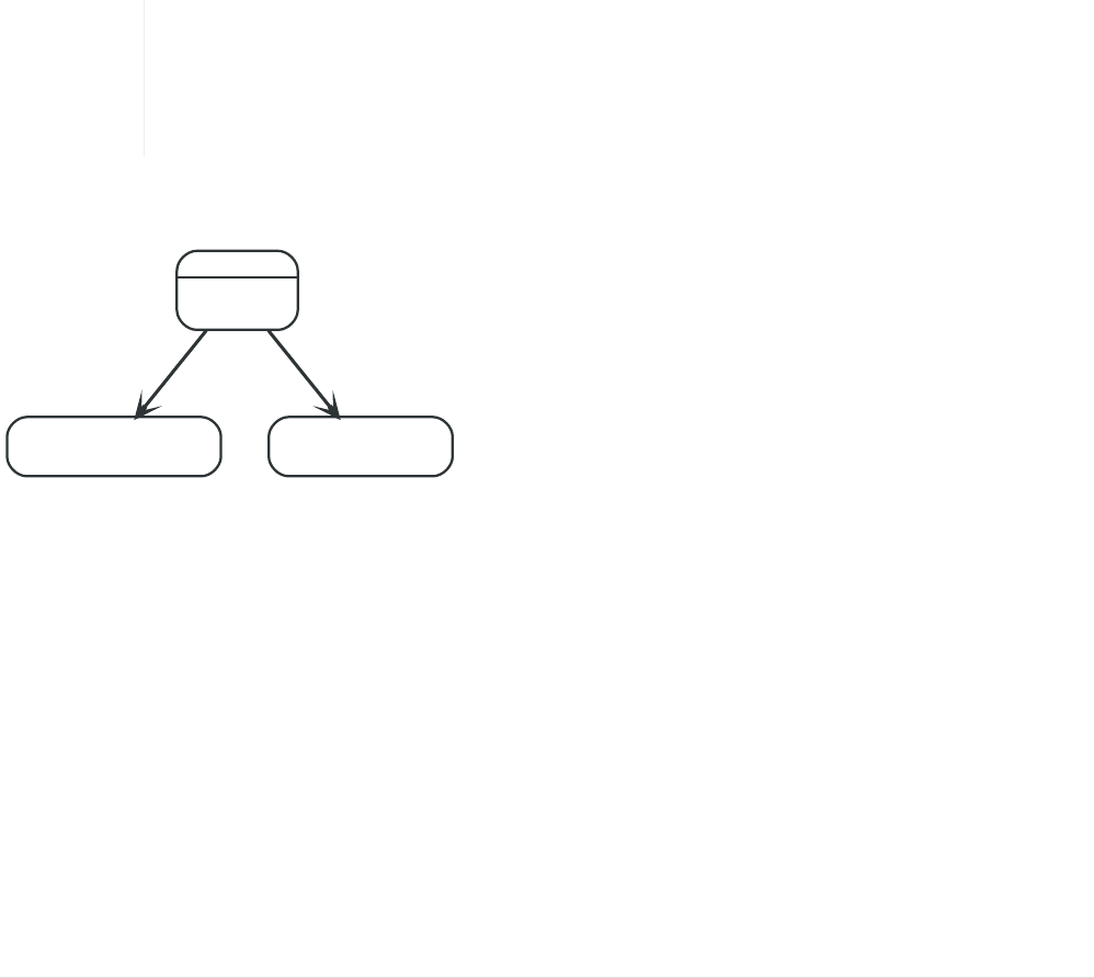
• IN operator
• Missing properties and values
• Default to false if property is missing
• Default to true if property is missing
• Filter on null
• Using ranges
• Simple range
• Composite range
Introduction
WHERE is not a clause in its own right — rather, it’s part of MATCH, OPTIONAL MATCH, START and WITH.
In the case of WITH and START, WHERE simply filters the results.
For MATCH and OPTIONAL MATCH on the other hand, WHERE adds constraints to the patterns described. It
should not be seen as a filter after the matching is finished.
In the case of multiple MATCH / OPTIONAL MATCH clauses, the predicate in WHERE is
always a part of the patterns in the directly preceding MATCH / OPTIONAL MATCH. Both
results and performance may be impacted if the WHERE is put inside the wrong
MATCH clause.
The following graph is used for the examples below:
Swedish
name = 'Andres'
age = 36
belt = 'white'
email = 'peter_n@example.com'
name = 'Peter'
age = 35
KNOWS
since = 1999
address = 'Sweden/Malmo'
name = 'Tobias'
age = 25
KNOWS
since = 2012
Figure 11. Graph
Basic usage
Boolean operations
You can use the boolean operators AND, OR, XOR and NOT. See Working with null for more information
on how this works with null.
84

Query
MATCH (n)
WHERE n.name = 'Peter' XOR (n.age < 30 AND n.name = 'Tobias') OR NOT (n.name =
'Tobias' OR n.name = 'Peter')
RETURN n.name, n.age
Table 73. Result
n.name n.age
"Andres" 36
"Tobias" 25
"Peter" 35
3 rows
Filter on node label
To filter nodes by label, write a label predicate after the WHERE keyword using WHERE n:foo.
Query
MATCH (n)
WHERE n:Swedish
RETURN n.name, n.age
The name and age for the 'Andres' node will be returned.
Table 74. Result
n.name n.age
"Andres" 36
1 row
Filter on node property
To filter on a node property, write your clause after the WHERE keyword.
Query
MATCH (n)
WHERE n.age < 30
RETURN n.name, n.age
The name and age values for the 'Tobias' node are returned because he is less than 30 years of age.
Table 75. Result
85

n.name n.age
"Tobias" 25
1 row
Filter on relationship property
To filter on a relationship property, write your clause after the WHERE keyword.
Query
MATCH (n)-[k:KNOWS]->(f)
WHERE k.since < 2000
RETURN f.name, f.age, f.email
The name, age and email values for the 'Peter' node are returned because Andrés has known him
since before 2000.
Table 76. Result
f.name f.age f.email
1 row
Filter on dynamically-computed node property
To filter on a property using a dynamically computed name, use square bracket syntax.
Query
WITH 'AGE' AS propname
MATCH (n)
WHERE n[toLower(propname)]< 30
RETURN n.name, n.age
The name and age values for the 'Tobias' node are returned because he is less than 30 years of age.
Table 77. Result
n.name n.age
"Tobias" 25
1 row
Property existence checking
Use the exists() function to only include nodes or relationships in which a property exists.
86

Query
MATCH (n)
WHERE exists(n.belt)
RETURN n.name, n.belt
The name and belt for the 'Andres' node are returned because he is the only one with a belt
property.
Table 78. Result
n.name n.belt
"Andres" "white"
1 row
String matching
The start and end of strings can be matched using STARTS WITH and ENDS WITH. To match regardless
of location in a string, use CONTAINS. The matching is case-sensitive.
Match the beginning of a string
The STARTS WITH operator is used to perform case-sensitive matching on the start of strings.
Query
MATCH (n)
WHERE n.name STARTS WITH 'Pet'
RETURN n.name, n.age
The name and age for the 'Peter' node are returned because his name starts with 'Pet'.
Table 79. Result
n.name n.age
"Peter" 35
1 row
Match the ending of a string
The ENDS WITH operator is used to perform case-sensitive matching on the end of strings.
Query
MATCH (n)
WHERE n.name ENDS WITH 'ter'
RETURN n.name, n.age
87

The name and age for the 'Peter' node are returned because his name ends with 'ter'.
Table 80. Result
n.name n.age
"Peter" 35
1 row
Match anywhere within a string
The CONTAINS operator is used to perform case-sensitive matching regardless of location in strings.
Query
MATCH (n)
WHERE n.name CONTAINS 'ete'
RETURN n.name, n.age
The name and age for the 'Peter' node are returned because his name contains with 'ete'.
Table 81. Result
n.name n.age
"Peter" 35
1 row
String matching negation
Use the NOT keyword to exclude all matches on given string from your result:
Query
MATCH (n)
WHERE NOT n.name ENDS WITH 's'
RETURN n.name, n.age
The name and age for the 'Peter' node are returned because his name does not end with 's'.
Table 82. Result
n.name n.age
"Peter" 35
1 row
Using path patterns in WHERE
88

Filter on patterns
Patterns are not only expressions, they are also predicates. The only limitation to your pattern is
that you must be able to express it in a single path. You cannot use commas between multiple paths
like you do in MATCH. You can achieve the same effect by combining multiple patterns with AND.
Note that you cannot introduce new variables here. Although it might look very similar to the MATCH
patterns, the WHERE clause is all about eliminating matched subgraphs. MATCH (a)-[*]->(b) is very
different from WHERE (a)-[*]->(b). The first will produce a subgraph for every path it can find
between a and b, whereas the latter will eliminate any matched subgraphs where a and b do not
have a directed relationship chain between them.
Query
MATCH (tobias {name: 'Tobias'}), (others)
WHERE others.name IN ['Andres', 'Peter'] AND (tobias)<-[]-(others)
RETURN others.name, others.age
The name and age for nodes that have an outgoing relationship to the 'Tobias' node are returned.
Table 83. Result
others.name others.age
"Andres" 36
1 row
Filter on patterns using NOT
The NOT operator can be used to exclude a pattern.
Query
MATCH (persons), (peter {name: 'Peter'})
WHERE NOT (persons)-[]->(peter)
RETURN persons.name, persons.age
Name and age values for nodes that do not have an outgoing relationship to the 'Peter' node are
returned.
Table 84. Result
persons.name persons.age
"Tobias" 25
"Peter" 35
2 rows
89

Filter on patterns with properties
You can also add properties to your patterns:
Query
MATCH (n)
WHERE (n)-[:KNOWS]-({name: 'Tobias'})
RETURN n.name, n.age
Finds all name and age values for nodes that have a KNOWS relationship to a node with the name
'Tobias'.
Table 85. Result
n.name n.age
"Andres" 36
1 row
Filter on relationship type
You can put the exact relationship type in the MATCH pattern, but sometimes you want to be able to
do more advanced filtering on the type. You can use the special property type to compare the type
with something else.
Query
MATCH (n)-[r]->()
WHERE n.name='Andres' AND type(r) STARTS WITH 'K'
RETURN type(r), r.since
This returns all relationships having a type whose name starts with 'K'.
Table 86. Result
type(r) r.since
"KNOWS" 1999
"KNOWS" 2012
2 rows
Lists
IN operator
To check if an element exists in a list, you can use the IN operator.
90

Query
MATCH (a)
WHERE a.name IN ['Peter', 'Tobias']
RETURN a.name, a.age
This query shows how to check if a property exists in a literal list.
Table 87. Result
a.name a.age
"Tobias" 25
"Peter" 35
2 rows
Missing properties and values
Default to false if property is missing
As missing properties evaluate to null, the comparision in the example will evaluate to false for
nodes without the belt property.
Query
MATCH (n)
WHERE n.belt = 'white'
RETURN n.name, n.age, n.belt
Only the name, age and belt values of nodes with white belts are returned.
Table 88. Result
n.name n.age n.belt
"Andres" 36 "white"
1 row
Default to true if property is missing
If you want to compare a property on a graph element, but only if it exists, you can compare the
property against both the value you are looking for and null, like:
Query
MATCH (n)
WHERE n.belt = 'white' OR n.belt IS NULL RETURN n.name, n.age, n.belt
ORDER BY n.name
91

This returns all values for all nodes, even those without the belt property.
Table 89. Result
n.name n.age n.belt
"Andres" 36 "white"
"Peter" 35 <null>
"Tobias" 25 <null>
3 rows
Filter on null
Sometimes you might want to test if a value or a variable is null. This is done just like SQL does it,
using IS NULL. Also like SQL, the negative is IS NOT NULL, although NOT(IS NULL x) also works.
Query
MATCH (person)
WHERE person.name = 'Peter' AND person.belt IS NULL RETURN person.name, person.age,
person.belt
The name and age values for nodes that have name 'Peter' but no belt property are returned.
Table 90. Result
person.name person.age person.belt
"Peter" 35 <null>
1 row
Using ranges
Simple range
To check for an element being inside a specific range, use the inequality operators <, <=, >=, >.
Query
MATCH (a)
WHERE a.name >= 'Peter'
RETURN a.name, a.age
The name and age values of nodes having a name property lexicographically greater than or equal
to 'Peter' are returned.
Table 91. Result
92

a.name a.age
"Tobias" 25
"Peter" 35
2 rows
Composite range
Several inequalities can be used to construct a range.
Query
MATCH (a)
WHERE a.name > 'Andres' AND a.name < 'Tobias'
RETURN a.name, a.age
The name and age values of nodes having a name property lexicographically between 'Andres' and
'Tobias' are returned.
Table 92. Result
a.name a.age
"Peter" 35
1 row
ORDER BY
ORDER BY is a sub-clause following RETURN or WITH, and it specifies that the
output should be sorted and how.
• Introduction
• Order nodes by property
• Order nodes by multiple properties
• Order nodes in descending order
• Ordering null
Introduction
Note that you cannot sort on nodes or relationships, just on properties on these. ORDER BY relies on
comparisons to sort the output, see Ordering and comparison of values.
In terms of scope of variables, ORDER BY follows special rules, depending on if the projecting RETURN
or WITH clause is either aggregating or DISTINCT. If it is an aggregating or DISTINCT projection, only
the variables available in the projection are available. If the projection does not alter the output
cardinality (which aggregation and DISTINCT do), variables available from before the projecting
93

clause are also available. When the projection clause shadows already existing variables, only the
new variables are available.
Lastly, it is not allowed to use aggregating expressions in the ORDER BY sub-clause if they are not also
listed in the projecting clause. This last rule is to make sure that ORDER BY does not change the
results, only the order of them.
name = 'A'
age = 34
length = 170
name = 'B'
age = 34
KNOWS
name = 'C'
age = 32
length = 185
KNOWS
Figure 12. Graph
Order nodes by property
ORDER BY is used to sort the output.
Query
MATCH (n)
RETURN n.name, n.age
ORDER BY n.name
The nodes are returned, sorted by their name.
Table 93. Result
n.name n.age
"A" 34
"B" 34
"C" 32
3 rows
Order nodes by multiple properties
You can order by multiple properties by stating each variable in the ORDER BY clause. Cypher will
sort the result by the first variable listed, and for equals values, go to the next property in the ORDER
BY clause, and so on.
94

Query
MATCH (n)
RETURN n.name, n.age
ORDER BY n.age, n.name
This returns the nodes, sorted first by their age, and then by their name.
Table 94. Result
n.name n.age
"C" 32
"A" 34
"B" 34
3 rows
Order nodes in descending order
By adding DESC[ENDING] after the variable to sort on, the sort will be done in reverse order.
Query
MATCH (n)
RETURN n.name, n.age
ORDER BY n.name DESC
The example returns the nodes, sorted by their name in reverse order.
Table 95. Result
n.name n.age
"C" 32
"B" 34
"A" 34
3 rows
Ordering null
When sorting the result set, null will always come at the end of the result set for ascending sorting,
and first when doing descending sort.
Query
MATCH (n)
RETURN n.length, n.name, n.age
ORDER BY n.length
95

The nodes are returned sorted by the length property, with a node without that property last.
Table 96. Result
n.length n.name n.age
170 "A" 34
185 "C" 32
<null> "B" 34
3 rows
SKIP
SKIP defines from which record to start including the records in the output.
• Introduction
• Skip first three records
• Return middle two records
• Using an expression with SKIP to return a subset of the records
Introduction
By using SKIP, the result set will get trimmed from the top. Please note that no guarantees are made
on the order of the result unless the query specifies the ORDER BY clause. SKIP accepts any expression
that evaluates to a positive integer — however the expression cannot refer to nodes or
relationships.
name = 'A'
name = 'E'
KNOWS
name = 'D'
KNOWS
name = 'C'
KNOWS
name = 'B'
KNOWS
Figure 13. Graph
Skip first three rows
To return a subset of the result, starting from the fourth result, use the following syntax:
Query
MATCH (n)
RETURN n.name
ORDER BY n.name
SKIP 3
96

The first three nodes are skipped, and only the last two are returned in the result.
Table 97. Result
n.name
"D"
"E"
2 rows
Return middle two rows
To return a subset of the result, starting from somewhere in the middle, use this syntax:
Query
MATCH (n)
RETURN n.name
ORDER BY n.name
SKIP 1
LIMIT 2
Two nodes from the middle are returned.
Table 98. Result
n.name
"B"
"C"
2 rows
Using an expression with SKIP to return a subset of the rows
Skip accepts any expression that evaluates to a positive integer as long as it is not referring to any
external variables:
Query
MATCH (n)
RETURN n.name
ORDER BY n.name
SKIP toInteger(3*rand())+ 1
The first three nodes are skipped, and only the last two are returned in the result.
Table 99. Result
97

n.name
"C"
"D"
"E"
3 rows
LIMIT
LIMIT constrains the number of records in the output.
• Introduction
• Return a subset of the records
• Using an expression with LIMIT to return a subset of the records
Introduction
LIMIT accepts any expression that evaluates to a positive integer — however the expression cannot
refer to nodes or relationships.
name = 'A'
name = 'E'
KNOWS
name = 'D'
KNOWS
name = 'C'
KNOWS
name = 'B'
KNOWS
Figure 14. Graph
Return a subset of the rows
To return a subset of the result, starting from the top, use this syntax:
Query
MATCH (n)
RETURN n.name
ORDER BY n.name
LIMIT 3
The top three items are returned by the example query.
Table 100. Result
n.name
"A"
"B"
98

n.name
"C"
3 rows
Using an expression with LIMIT to return a subset of the rows
Limit accepts any expression that evaluates to a positive integer as long as it is not referring to any
external variables:
Query
MATCH (n)
RETURN n.name
ORDER BY n.name
LIMIT toInteger(3 * rand())+ 1
Returns one to three top items.
Table 101. Result
n.name
"A"
"B"
2 rows
CREATE
The CREATE clause is used to create graph elements — nodes and
relationships.
• Create nodes
• Create single node
• Create multiple nodes
• Create a node with a label
• Create a node with multiple labels
• Create node and add labels and properties
• Return created node
• Create relationships
• Create a relationship between two nodes
• Create a relationship and set properties
99

•
Create a full path
• Use parameters with CREATE
• Create node with a parameter for the properties
• Create multiple nodes with a parameter for their properties
Create nodes
Create single node
Creating a single node is done by issuing the following query.
Query
CREATE (n)
Nothing is returned from this query, except the count of affected nodes.
Result
+-------------------+
| No data returned. |
+-------------------+
Nodes created: 1
Create multiple nodes
Creating multiple nodes is done by separating them with a comma.
Query
CREATE (n), (m)
Result
+-------------------+
| No data returned. |
+-------------------+
Nodes created: 2
Create a node with a label
To add a label when creating a node, use the syntax below.
Query
CREATE (n:Person)
100

Nothing is returned from this query.
Result
+-------------------+
| No data returned. |
+-------------------+
Nodes created: 1
Labels added: 1
Create a node with multiple labels
To add labels when creating a node, use the syntax below. In this case, we add two labels.
Query
CREATE (n:Person:Swedish)
Nothing is returned from this query.
Result
+-------------------+
| No data returned. |
+-------------------+
Nodes created: 1
Labels added: 2
Create node and add labels and properties
When creating a new node with labels, you can add properties at the same time.
Query
CREATE (n:Person {name: 'Andres', title: 'Developer'})
Nothing is returned from this query.
Result
+-------------------+
| No data returned. |
+-------------------+
Nodes created: 1
Properties set: 2
Labels added: 1
101

Return created node
Creating a single node is done by issuing the following query.
Query
CREATE (a {name: 'Andres'})
RETURN a
The newly-created node is returned.
Result
+------------------------+
| a |
+------------------------+
| Node[0]{name:"Andres"} |
+------------------------+
1 row
Nodes created: 1
Properties set: 1
Create relationships
Create a relationship between two nodes
To create a relationship between two nodes, we first get the two nodes. Once the nodes are loaded,
we simply create a relationship between them.
Query
MATCH (a:Person), (b:Person)
WHERE a.name = 'Node A' AND b.name = 'Node B'
CREATE (a)-[r:RELTYPE]->(b)
RETURN r
The created relationship is returned by the query.
Result
+---------------+
| r |
+---------------+
| :RELTYPE[0]{} |
+---------------+
1 row
Relationships created: 1
102

Create a relationship and set properties
Setting properties on relationships is done in a similar manner to how it’s done when creating
nodes. Note that the values can be any expression.
Query
MATCH (a:Person), (b:Person)
WHERE a.name = 'Node A' AND b.name = 'Node B'
CREATE (a)-[r:RELTYPE {name: a.name + '<->' + b.name}]->(b)
RETURN r
The newly-created relationship is returned by the example query.
Result
+-------------------------------------+
| r |
+-------------------------------------+
| :RELTYPE[0]{name:"Node A<->Node B"} |
+-------------------------------------+
1 row
Relationships created: 1
Properties set: 1
Create a full path
When you use CREATE and a pattern, all parts of the pattern that are not already in scope at this time
will be created.
Query
CREATE p = (andres {name:'Andres'})-[:WORKS_AT]->(neo)<-[:WORKS_AT]-(michael {name:
'Michael'})
RETURN p
This query creates three nodes and two relationships in one go, assigns it to a path variable, and
returns it.
103

Result
+-------------------------------------------------------------------------------------
-----+
| p
|
+-------------------------------------------------------------------------------------
-----+
|
[Node[0]{name:"Andres"},:WORKS_AT[0]{},Node[1]{},:WORKS_AT[1]{},Node[2]{name:"Michael"
}] |
+-------------------------------------------------------------------------------------
-----+
1 row
Nodes created: 3
Relationships created: 2
Properties set: 2
Use parameters with CREATE
Create node with a parameter for the properties
You can also create a graph entity from a map. All the key/value pairs in the map will be set as
properties on the created relationship or node. In this case we add a Person label to the node as
well.
Parameters
{
Ê "props" : {
Ê "name" : "Andres",
Ê "position" : "Developer"
Ê }
}
Query
CREATE (n:Person $props)
RETURN n
104

Result
+---------------------------------------------+
| n |
+---------------------------------------------+
| Node[0]{name:"Andres",position:"Developer"} |
+---------------------------------------------+
1 row
Nodes created: 1
Properties set: 2
Labels added: 1
Create multiple nodes with a parameter for their properties
By providing Cypher an array of maps, it will create a node for each map.
Parameters
{
Ê "props" : [ {
Ê "name" : "Andres",
Ê "position" : "Developer"
Ê }, {
Ê "name" : "Michael",
Ê "position" : "Developer"
Ê } ]
}
Query
UNWIND $props AS map
CREATE (n)
SET n = map
Result
+-------------------+
| No data returned. |
+-------------------+
Nodes created: 2
Properties set: 4
DELETE
The DELETE clause is used to delete graph elements — nodes, relationships or
paths.
105

• Introduction
• Delete a single node
• Delete all nodes and relationships
• Delete a node with all its relationships
• Delete relationships only
Introduction
For removing properties and labels, see REMOVE. Remember that you cannot delete a node without
also deleting relationships that start or end on said node. Either explicitly delete the relationships,
or use DETACH DELETE.
The examples start out with the following database:
name = 'Andres'
age = 36
name = 'Peter'
age = 34
KNOWS
name = 'Tobias'
age = 25
KNOWS
Delete single node
To delete a node, use the DELETE clause.
Query
MATCH (n:Useless)
DELETE n
Result
+-------------------+
| No data returned. |
+-------------------+
Nodes deleted: 1
Delete all nodes and relationships
This query isn’t for deleting large amounts of data, but is nice when playing around with small
example data sets.
Query
MATCH (n)
DETACH DELETE n
106

Result
+-------------------+
| No data returned. |
+-------------------+
Nodes deleted: 3
Relationships deleted: 2
Delete a node with all its relationships
When you want to delete a node and any relationship going to or from it, use DETACH DELETE.
Query
MATCH (n {name: 'Andres'})
DETACH DELETE n
Result
+-------------------+
| No data returned. |
+-------------------+
Nodes deleted: 1
Relationships deleted: 2
Delete relationships only
It is also possible to delete relationships only, leaving the node(s) otherwise unaffected.
Query
MATCH (n {name: 'Andres'})-[r:KNOWS]->()
DELETE r
This deletes all outgoing KNOWS relationships from the node with the name 'Andres'.
Result
+-------------------+
| No data returned. |
+-------------------+
Relationships deleted: 2
SET
The SET clause is used to update labels on nodes and properties on nodes
107

and relationships.
• Introduction
• Set a property
• Remove a property
• Copying properties between nodes and relationships
• Adding properties from maps
• Set a property using a parameter
• Set all properties using a parameter
• Set multiple properties using one SET clause
• Set a label on a node
• Set multiple labels on a node
Introduction
SET can also be used with maps from parameters to set properties.
Setting labels on a node is an idempotent operations — if you try to set a label on
a node that already has that label on it, nothing happens.
The examples use this graph as a starting point:
Swedish
name = 'Andres'
age = 36
hungry = true
name = 'Peter'
age = 34
KNOWS
name = 'Emil'
KNOWS
name = 'Stefan'
KNOWS
Set a property
To set a property on a node or relationship, use SET.
Query
MATCH (n {name: 'Andres'})
SET n.surname = 'Taylor'
RETURN n
The newly changed node is returned by the query.
108

Result
+------------------------------------------------------------+
| n |
+------------------------------------------------------------+
| Node[0]{surname:"Taylor",name:"Andres",age:36,hungry:true} |
+------------------------------------------------------------+
1 row
Properties set: 1
Remove a property
Normally you remove a property by using REMOVE, but it’s sometimes handy to do it using the SET
command. One example is if the property comes from a parameter.
Query
MATCH (n {name: 'Andres'})
SET n.name = NULL
RETURN n
The node is returned by the query, and the name property is now missing.
Result
+-----------------------------+
| n |
+-----------------------------+
| Node[0]{hungry:true,age:36} |
+-----------------------------+
1 row
Properties set: 1
Copying properties between nodes and relationships
You can also use SET to copy all properties from one graph element to another. Remember that
doing this will remove all other properties on the receiving graph element.
Query
MATCH (at {name: 'Andres'}), (pn {name: 'Peter'})
SET at = pn
RETURN at, pn
The 'Andres' node has had all its properties replaced by the properties in the 'Peter' node.
109

Result
+-------------------------------------------------------------+
| at | pn |
+-------------------------------------------------------------+
| Node[0]{name:"Peter",age:34} | Node[2]{name:"Peter",age:34} |
+-------------------------------------------------------------+
1 row
Properties set: 3
Adding properties from maps
When setting properties from a map (literal, parameter, or graph element), you can use the += form
of SET to only add properties, and not remove any of the existing properties on the graph element.
Query
MATCH (peter {name: 'Peter'})
SET peter += {hungry: TRUE, position: 'Entrepreneur'}
Result
+-------------------+
| No data returned. |
+-------------------+
Properties set: 2
Set a property using a parameter
Use a parameter to give the value of a property.
Parameters
{
Ê "surname" : "Taylor"
}
Query
MATCH (n {name: 'Andres'})
SET n.surname = $surname
RETURN n
The 'Andres' node has got a surname added.
110

Result
+------------------------------------------------------------+
| n |
+------------------------------------------------------------+
| Node[0]{surname:"Taylor",name:"Andres",age:36,hungry:true} |
+------------------------------------------------------------+
1 row
Properties set: 1
Set all properties using a parameter
This will replace all existing properties on the node with the new set provided by the parameter.
Parameters
{
Ê "props" : {
Ê "name" : "Andres",
Ê "position" : "Developer"
Ê }
}
Query
MATCH (n {name: 'Andres'})
SET n = $props
RETURN n
The 'Andres' node has had all its properties replaced by the properties in the props parameter.
Result
+---------------------------------------------+
| n |
+---------------------------------------------+
| Node[0]{name:"Andres",position:"Developer"} |
+---------------------------------------------+
1 row
Properties set: 4
Set multiple properties using one SET clause
If you want to set multiple properties in one go, simply separate them with a comma.
111

Query
MATCH (n {name: 'Andres'})
SET n.position = 'Developer', n.surname = 'Taylor'
Result
+-------------------+
| No data returned. |
+-------------------+
Properties set: 2
Set a label on a node
To set a label on a node, use SET.
Query
MATCH (n {name: 'Stefan'})
SET n:German
RETURN n
The newly labeled node is returned by the query.
Result
+------------------------+
| n |
+------------------------+
| Node[3]{name:"Stefan"} |
+------------------------+
1 row
Labels added: 1
Set multiple labels on a node
To set multiple labels on a node, use SET and separate the different labels using :.
Query
MATCH (n {name: 'Emil'})
SET n:Swedish:Bossman
RETURN n
The newly labeled node is returned by the query.
112

Result
+----------------------+
| n |
+----------------------+
| Node[1]{name:"Emil"} |
+----------------------+
1 row
Labels added: 2
REMOVE
The REMOVE clause is used to remove properties and labels from graph
elements.
• Introduction
• Remove a property
• Remove a label from a node
• Removing multiple labels
Introduction
For deleting nodes and relationships, see DELETE.
Removing labels from a node is an idempotent operation: If you try to remove a
label from a node that does not have that label on it, nothing happens.
The examples use the following database:
Swedish
name = 'Andres'
age = 36
Swedish, German
name = 'Peter'
age = 34
KNOWS
Swedish
name = 'Tobias'
age = 25
KNOWS
Remove a property
Cypher doesn’t allow storing null in properties. Instead, if no value exists, the property is just not
there. So, to remove a property value on a node or a relationship, is also done with REMOVE.
113

Query
MATCH (andres {name: 'Andres'})
REMOVE andres.age
RETURN andres
The node is returned, and no property age exists on it.
Result
+------------------------+
| andres |
+------------------------+
| Node[0]{name:"Andres"} |
+------------------------+
1 row
Properties set: 1
Remove a label from a node
To remove labels, you use REMOVE.
Query
MATCH (n {name: 'Peter'})
REMOVE n:German
RETURN n
Result
+------------------------------+
| n |
+------------------------------+
| Node[2]{name:"Peter",age:34} |
+------------------------------+
1 row
Labels removed: 1
Removing multiple labels
To remove multiple labels, you use REMOVE.
Query
MATCH (n {name: 'Peter'})
REMOVE n:German:Swedish
RETURN n
114

Result
+------------------------------+
| n |
+------------------------------+
| Node[2]{name:"Peter",age:34} |
+------------------------------+
1 row
Labels removed: 2
MERGE
The MERGE clause ensures that a pattern exists in the graph. Either the
pattern already exists, or it needs to be created.
• Introduction
• Merge nodes
• Merge single node with a label
• Merge single node with properties
• Merge single node specifying both label and property
• Merge single node derived from an existing node property
• Merge relationships
• Merge on a relationship
• Merge on multiple relationships
• Merge on an undirected relationship
• Merge on a relationship between two existing nodes
• Merge on a relationship between an existing node and a merged node derived from a node
property
• Using map parameters with MERGE
Introduction
MERGE either matches existing nodes and binds them, or it creates new data and binds that. It’s like a
combination of MATCH and CREATE that additionally allows you to specify what happens if the data
was matched or created.
For example, you can specify that the graph must contain a node for a user with a certain name. If
there isn’t a node with the correct name, a new node will be created and its name property set.
When using MERGE on full patterns, the behavior is that either the whole pattern matches, or the
whole pattern is created. MERGE will not partially use existing patterns — it’s all or nothing. If partial
matches are needed, this can be accomplished by splitting a pattern up into multiple MERGE clauses.
115

As with MATCH, MERGE can match multiple occurrences of a pattern. If there are multiple matches,
they will all be passed on to later stages of the query.
The following graph is used for the examples below:
Movie
name = 'WallStreet'
title = 'Wall Street'
Person
chauffeurName = 'Ted Green'
name = 'Rob Reiner'
bornIn = 'New York'
Movie
title = 'The American President'
name = 'TheAmericanPresident'
DIRECTED
Person
chauffeurName = 'Bill White'
name = 'Oliver Stone'
bornIn = 'New York'
DIRECTED
Person
chauffeurName = 'John Brown'
name = 'Charlie Sheen'
bornIn = 'New York'
ACTED_IN
Person
chauffeurName = 'Bob Brown'
name = 'Martin Sheen'
bornIn = 'Ohio'
FATHER
ACTED_IN ACTED_IN
Person
bornIn = 'New Jersey'
chauffeurName = 'John Brown'
name = 'Michael Douglas'
ACTED_IN ACTED_IN
Figure 15. Graph
Merge nodes
Merge single node with a label
Merging a single node with the given label.
Query
MERGE (robert:Critic)
RETURN robert, labels(robert)
A new node is created because there are no nodes labeled Critic in the database.
Result
+----------------------------+
| robert | labels(robert) |
+----------------------------+
| Node[7]{} | ["Critic"] |
+----------------------------+
1 row
Nodes created: 1
Labels added: 1
Merge single node with properties
Merging a single node with properties where not all properties match any existing node.
Query
MERGE (charlie {name: 'Charlie Sheen', age: 10})
RETURN charlie
116

A new node with the name 'Charlie Sheen' will be created since not all properties matched the
existing 'Charlie Sheen' node.
Result
+--------------------------------------+
| charlie |
+--------------------------------------+
| Node[7]{name:"Charlie Sheen",age:10} |
+--------------------------------------+
1 row
Nodes created: 1
Properties set: 2
Merge single node specifying both label and property
Merging a single node with both label and property matching an existing node.
Query
MERGE (michael:Person {name: 'Michael Douglas'})
RETURN michael.name, michael.bornIn
'Michael Douglas' will be matched and the name and bornIn properties returned.
Result
+------------------------------------+
| michael.name | michael.bornIn |
+------------------------------------+
| "Michael Douglas" | "New Jersey" |
+------------------------------------+
1 row
Merge single node derived from an existing node property
For some property 'p' in each bound node in a set of nodes, a single new node is created for each
unique value for 'p'.
Query
MATCH (person:Person)
MERGE (city:City {name: person.bornIn})
RETURN person.name, person.bornIn, city
Three nodes labeled City are created, each of which contains a name property with the value of
'New York', 'Ohio', and 'New Jersey', respectively. Note that even though the MATCH clause results in
three bound nodes having the value 'New York' for the bornIn property, only a single 'New York'
117

node (i.e. a City node with a name of 'New York') is created. As the 'New York' node is not matched
for the first bound node, it is created. However, the newly-created 'New York' node is matched and
bound for the second and third bound nodes.
Result
+----------------------------------------------------------------+
| person.name | person.bornIn | city |
+----------------------------------------------------------------+
| "Rob Reiner" | "New York" | Node[7]{name:"New York"} |
| "Oliver Stone" | "New York" | Node[7]{name:"New York"} |
| "Charlie Sheen" | "New York" | Node[7]{name:"New York"} |
| "Michael Douglas" | "New Jersey" | Node[8]{name:"New Jersey"} |
| "Martin Sheen" | "Ohio" | Node[9]{name:"Ohio"} |
+----------------------------------------------------------------+
5 rows
Nodes created: 3
Properties set: 3
Labels added: 3
Merge relationships
Merge on a relationship
MERGE can be used to match or create a relationship.
Query
MATCH (charlie:Person {name: 'Charlie Sheen'}), (wallStreet:Movie {title: 'Wall
Street'})
MERGE (charlie)-[r:ACTED_IN]->(wallStreet)
RETURN charlie.name, type(r), wallStreet.title
'Charlie Sheen' had already been marked as acting in 'Wall Street', so the existing relationship is
found and returned. Note that in order to match or create a relationship when using MERGE, at least
one bound node must be specified, which is done via the MATCH clause in the above example.
Result
+-------------------------------------------------+
| charlie.name | type(r) | wallStreet.title |
+-------------------------------------------------+
| "Charlie Sheen" | "ACTED_IN" | "Wall Street" |
+-------------------------------------------------+
1 row
Merge on multiple relationships
When MERGE is used on a whole pattern, either everything matches, or everything is created.
118

Query
MATCH (oliver:Person {name: 'Oliver Stone'}), (reiner:Person {name: 'Rob Reiner'})
MERGE (oliver)-[:DIRECTED]->(movie:Movie)<-[:ACTED_IN]-(reiner)
RETURN movie
In our example graph, 'Oliver Stone' and 'Rob Reiner' have never worked together. When we try
to MERGE a movie between them, Cypher will not use any of the existing movies already connected to
either person. Instead, a new 'movie' node is created.
Result
+-----------+
| movie |
+-----------+
| Node[7]{} |
+-----------+
1 row
Nodes created: 1
Relationships created: 2
Labels added: 1
Merge on an undirected relationship
MERGE can also be used with an undirected relationship. When it needs to create a new one, it will
pick a direction.
Query
MATCH (charlie:Person {name: 'Charlie Sheen'}), (oliver:Person {name: 'Oliver Stone'})
MERGE (charlie)-[r:KNOWS]-(oliver)
RETURN r
As 'Charlie Sheen' and 'Oliver Stone' do not know each other, this MERGE query will create a KNOWS
relationship between them. The direction of the created relationship is arbitrary.
Result
+-------------+
| r |
+-------------+
| :KNOWS[8]{} |
+-------------+
1 row
Relationships created: 1
119

Merge on a relationship between two existing nodes
MERGE can be used in conjunction with preceding MATCH and MERGE clauses to create a relationship
between two bound nodes 'm' and 'n', where 'm' is returned by MATCH and 'n' is created or matched
by the earlier MERGE.
Query
MATCH (person:Person)
MERGE (city:City {name: person.bornIn})
MERGE (person)-[r:BORN_IN]->(city)
RETURN person.name, person.bornIn, city
This builds on the example from Merge single node derived from an existing node property. The
second MERGE creates a BORN_IN relationship between each person and a city corresponding to the
value of the person’s bornIn property. 'Charlie Sheen', 'Rob Reiner' and 'Oliver Stone' all have a
BORN_IN relationship to the 'same' City node ('New York').
Result
+----------------------------------------------------------------+
| person.name | person.bornIn | city |
+----------------------------------------------------------------+
| "Rob Reiner" | "New York" | Node[7]{name:"New York"} |
| "Oliver Stone" | "New York" | Node[7]{name:"New York"} |
| "Charlie Sheen" | "New York" | Node[7]{name:"New York"} |
| "Michael Douglas" | "New Jersey" | Node[8]{name:"New Jersey"} |
| "Martin Sheen" | "Ohio" | Node[9]{name:"Ohio"} |
+----------------------------------------------------------------+
5 rows
Nodes created: 3
Relationships created: 5
Properties set: 3
Labels added: 3
Merge on a relationship between an existing node and a merged node derived from a node
property
MERGE can be used to simultaneously create both a new node 'n' and a relationship between a bound
node 'm' and 'n'.
Query
MATCH (person:Person)
MERGE (person)-[r:HAS_CHAUFFEUR]->(chauffeur:Chauffeur {name: person.chauffeurName})
RETURN person.name, person.chauffeurName, chauffeur
As MERGE found no matches — in our example graph, there are no nodes labeled with Chauffeur and
no HAS_CHAUFFEUR relationships — MERGE creates five nodes labeled with Chauffeur, each of which
120

contains a name property whose value corresponds to each matched Person node’s chauffeurName
property value. MERGE also creates a HAS_CHAUFFEUR relationship between each Person node and the
newly-created corresponding Chauffeur node. As 'Charlie Sheen' and 'Michael Douglas' both have
a chauffeur with the same name — 'John Brown' — a new node is created in each case, resulting in
'two' Chauffeur nodes having a name of 'John Brown', correctly denoting the fact that even though
the name property may be identical, these are two separate people. This is in contrast to the example
shown above in Merge on a relationship between two existing nodes, where we used the first MERGE
to bind the City nodes to prevent them from being recreated (and thus duplicated) in the second
MERGE.
Result
+------------------------------------------------------------------------+
| person.name | person.chauffeurName | chauffeur |
+------------------------------------------------------------------------+
| "Rob Reiner" | "Ted Green" | Node[7]{name:"Ted Green"} |
| "Oliver Stone" | "Bill White" | Node[8]{name:"Bill White"} |
| "Charlie Sheen" | "John Brown" | Node[9]{name:"John Brown"} |
| "Michael Douglas" | "John Brown" | Node[10]{name:"John Brown"} |
| "Martin Sheen" | "Bob Brown" | Node[11]{name:"Bob Brown"} |
+------------------------------------------------------------------------+
5 rows
Nodes created: 5
Relationships created: 5
Properties set: 5
Labels added: 5
Using map parameters with MERGE
MERGE does not support map parameters the same way CREATE does. To use map parameters with
MERGE, it is necessary to explicitly use the expected properties, such as in the following example. For
more information on parameters, see Parameters.
Parameters
{
Ê "param" : {
Ê "name" : "Keanu Reeves",
Ê "role" : "Neo"
Ê }
}
Query
MERGE (person:Person {name: $param.name, role: $param.role})
RETURN person.name, person.role
121

Result
+------------------------------+
| person.name | person.role |
+------------------------------+
| "Keanu Reeves" | "Neo" |
+------------------------------+
1 row
Nodes created: 1
Properties set: 2
Labels added: 1
CALL[…YIELD]
The CALL clause is used to call a procedure deployed in the database.
• Introduction
• Call a procedure using CALL
• View the signature for a procedure
• Call a procedure using a quoted namespace and name
• Call a procedure with literal arguments
• Call a procedure with parameter arguments
• Call a procedure with mixed literal and parameter arguments
• Call a procedure with literal and default arguments
• Call a procedure within a complex query using CALL…YIELD
• Call a procedure and filter its results
• Call a procedure within a complex query and rename its outputs
Introduction
Procedures are called using the CALL clause.
Each procedure call needs to specify all required procedure arguments. This may be done either
explicitly, by using a comma-separated list wrapped in parentheses after the procedure name, or
implicitly by using available query parameters as procedure call arguments. The latter form is
available only in a so-called standalone procedure call, when the whole query consists of a single
CALL clause.
Most procedures return a stream of records with a fixed set of result fields, similar to how running
a Cypher query returns a stream of records. The YIELD sub-clause is used to explicitly select which
of the available result fields are returned as newly-bound variables from the procedure call to the
user or for further processing by the remaining query. Thus, in order to be able to use YIELD, the
names (and types) of the output parameters need be known in advance. Each yielded result field
may optionally be renamed using aliasing (i.e. resultFieldName AS newName). All new variables
122

bound by a procedure call are added to the set of variables already bound in the current scope. It is
an error if a procedure call tries to rebind a previously bound variable (i.e. a procedure call cannot
shadow a variable that was previously bound in the current scope).
This section explains how to determine a procedure’s input parameters (needed for CALL) and
output parameters (needed for YIELD).
Inside a larger query, the records returned from a procedure call with an explicit YIELD may be
further filtered using a WHERE sub-clause followed by a predicate (similar to WITH … WHERE …).
If the called procedure declares at least one result field, YIELD may generally not be omitted.
However YIELD may always be omitted in a standalone procedure call. In this case, all result fields
are yielded as newly-bound variables from the procedure call to the user.
Cypher supports the notion of VOID procedures. A VOID procedure is a procedure that does not
declare any result fields and returns no result records and that has explicitly been declared as VOID.
Calling a VOID procedure may only have a side effect and thus does neither allow nor require the
use of YIELD. Calling a VOID procedure in the middle of a larger query will simply pass on each input
record (i.e. it acts like WITH * in terms of the record stream).
This clause cannot be combined with other clauses.
Call a procedure using CALL
This calls a procedure db.labels, which lists all labels used in the database.
Query
CALL db.labels
Result
+-----------------+
| label |
+-----------------+
| "User" |
| "Administrator" |
+-----------------+
2 rows
View the signature for a procedure
To CALL a procedure, its input parameters need to be known, and to use YIELD, its output parameters
need to be known. A procedure dbms.procedures returns the name, signature and description for all
procedures. The following query can be used to return the signature for a particular procedure:
123

Query
CALL dbms.procedures() YIELD name, signature
WHERE name='dbms.listConfig'
RETURN signature
We can see that the dbms.listConfig has one input parameter, searchString, and three output
parameters, name, description and value.
Result
+-------------------------------------------------------------------------------------
-------------------------+
| signature
|
+-------------------------------------------------------------------------------------
-------------------------+
| "dbms.listConfig(searchString = :: STRING?) :: (name :: STRING?, description ::
STRING?, value :: STRING?)" |
+-------------------------------------------------------------------------------------
-------------------------+
1 row
Call a procedure using a quoted namespace and name
This calls a procedure db.labels, which lists all labels used in the database.
Query
CALL `db`.`labels`
Result
+-----------------+
| label |
+-----------------+
| "User" |
| "Administrator" |
+-----------------+
2 rows
Call a procedure with literal arguments
This calls the example procedure org.opencypher.procedure.example.addNodeToIndex using literal
arguments, i.e. arguments that are written out directly in the statement text.
124

Query
CALL org.opencypher.procedure.example.addNodeToIndex('users', 0, 'name')
Since our example procedure does not return any result, the result is empty.
Result
+--------------------------------------------+
| No data returned, and nothing was changed. |
+--------------------------------------------+
Call a procedure with parameter arguments
This calls the example procedure org.opencypher.procedure.example.addNodeToIndex using
parameters as arguments. Each procedure argument is taken to be the value of a corresponding
statement parameters with the same name (or null if no such parameter has been given).
Parameters
{
Ê "indexName" : "users",
Ê "node" : 0,
Ê "propKey" : "name"
}
Query
CALL org.opencypher.procedure.example.addNodeToIndex
Since our example procedure does not return any result, the result is empty.
Result
+--------------------------------------------+
| No data returned, and nothing was changed. |
+--------------------------------------------+
Call a procedure with mixed literal and parameter arguments
This calls the example procedure org.opencypher.procedure.example.addNodeToIndex using both
literal and parameter arguments.
125

Parameters
{
Ê "node" : 0
}
Query
CALL org.opencypher.procedure.example.addNodeToIndex('users', $node, 'name')
Since our example procedure does not return any result, the result is empty.
Result
+--------------------------------------------+
| No data returned, and nothing was changed. |
+--------------------------------------------+
Call a procedure with literal and default arguments
This calls the example procedure org.opencypher.procedure.example.addNodeToIndex using literal
arguments, i.e. arguments that are written out directly in the statement text, and a trailing default
argument that is provided by the procedure itself.
Query
CALL org.opencypher.procedure.example.addNodeToIndex('users', 0)
Since our example procedure does not return any result, the result is empty.
Result
+--------------------------------------------+
| No data returned, and nothing was changed. |
+--------------------------------------------+
Call a procedure within a complex query using CALL YIELD
This calls a procedure db.labels to count all labels used in the database.
Query
CALL db.labels() YIELD label
RETURN count(label) AS numLabels
Since the procedure call is part of a larger query, all outputs must be named explicitly.
126

Result
+-----------+
| numLabels |
+-----------+
| 2 |
+-----------+
1 row
Call a procedure and filter its results
This calls a procedure db.labels to count all in-use labels in the database that contain the word
'User'
Query
CALL db.labels() YIELD label
WHERE label CONTAINS 'User'
RETURN count(label) AS numLabels
Since the procedure call is part of a larger query, all outputs must be named explicitly.
Result
+-----------+
| numLabels |
+-----------+
| 1 |
+-----------+
1 row
Call a procedure within a complex query and rename its outputs
This calls a procedure db.propertyKeys as part of counting the number of nodes per property key
that is currently used in the database.
Query
CALL db.propertyKeys() YIELD propertyKey AS prop
MATCH (n)
WHERE n[prop] IS NOT NULL RETURN prop, count(n) AS numNodes
Since the procedure call is part of a larger query, all outputs must be named explicitly.
127

Result
+-------------------+
| prop | numNodes |
+-------------------+
| "name" | 1 |
+-------------------+
1 row
UNION
The UNION clause is used to combine the result of multiple queries.
• Introduction
• Combine two queries and retain duplicates
• Combine two queries and remove duplicates
Introduction
UNION combines the results of two or more queries into a single result set that includes all the
records that belong to all queries in the union.
The number and the names of the fields must be identical in all queries combined by using UNION.
To keep all the result records, use UNION ALL. Using just UNION will combine and remove duplicates
from the result set.
Actor
name = 'Anthony Hopkins'
Movie
title = 'Hitchcock'
ACTS_IN
Actor
name = 'Helen Mirren'
KNOWS
ACTS_IN
Actor
name = 'Hitchcock'
Figure 16. Graph
Combine two queries and retain duplicates
Combining the results from two queries is done using UNION ALL.
128

Query
MATCH (n:Actor)
RETURN n.name AS name
UNION ALL MATCH (n:Movie)
RETURN n.title AS name
The combined result is returned, including duplicates.
Table 102. Result
name
"Anthony Hopkins"
"Helen Mirren"
"Hitchcock"
"Hitchcock"
4 rows
Combine two queries and remove duplicates
By not including ALL in the UNION, duplicates are removed from the combined result set
Query
MATCH (n:Actor)
RETURN n.name AS name
UNION
MATCH (n:Movie)
RETURN n.title AS name
The combined result is returned, without duplicates.
Table 103. Result
name
"Anthony Hopkins"
"Helen Mirren"
"Hitchcock"
3 rows
State visibility and behaviour between clauses
• Introduction
• Examples
129

Introduction
Cypher allows clauses that read from the graph to be interleaved with clauses that write to the
graph. Some clauses can also do both - read the graph and write to it at the same time. Explicit state
change visibility makes it possible to understand queries without having to worry about ordering
of updates and reads. The semantics of the data flow here is such that each clause operates on the
entire result set before passing control to any subsequent clause. From an implementation
perspective, these semantics also allow us to make some queries more performant than they can be
today, by ignoring statement state for a lot of graph reading, and saving us from eagerly producing
matching results before updates can be applied.
We call the concept discussed eagerness. This means that each clause logically consumes all
incoming rows eagerly, and only produces output when the input is exhausted. This concept is in
contrast to lazy evaluation (https://en.wikipedia.org/wiki/Lazy_evaluation), which, when applied to
Cypher, means that each clause only processes as much input as is necessary for the first record of
output to be sent to the subsequent clause.
Each clause lives in its own state, which includes all the changes of clauses coming before it,
including changes performed by itself, but none of the changes made by clauses listed later in
the query.
Updates between UNION subqueries are also treated in a sequential manner. Therefore subqueries
coming later will see updates from subqueries before, but not the other way around.
This is not about concurrency - even in a single user system this would need to be
thought through and defined explicitly.
Examples
Example query 1:
The following query would lead to a never-ending loop, if a lazy MATCH clause is not isolated from
the new nodes created by CREATE.
Query
MATCH (a)
CREATE ()
Example query 2:
Given a database containing two nodes, we illustrate the subtleties of query execution with the
following query.
130

Query
MATCH ()
CREATE ()
WITH *
MATCH ()
CREATE ()
Query Pre-existing nodes Rows in Nodes created Rows out
MATCH ()
2 1 0 2 (N)
CREATE ()
2 2 2 (R) 2
WITH *
4 2 0 2
MATCH ()
4 2 0 8 (N * R)
CREATE ()
4 8 8 8
Outcome 12 (2 + 2 + 8) - 10 8
Example query 3:
In the following query, the MATCH following the UNION will find the nodes created before the UNION.
Query
CREATE (a:X)
RETURN a AS column
UNION
MATCH (x:X)
CREATE ()
RETURN x as column
131

Functions
• Predicate functions [Summary|Detail]
• Scalar functions [Summary|Detail]
• Aggregating functions [Summary|Detail]
• List functions [Summary|Detail]
• Mathematical functions - numeric [Summary|Detail]
• Mathematical functions - logarithmic [Summary|Detail]
• Mathematical functions - trigonometric [Summary|Detail]
• String functions [Summary|Detail]
• User-defined functions
Note that related information exists in Operators.
Most functions in Cypher will return null if an input parameter is null.
Predicate functions
These functions return either true or false for the given arguments.
Function Description
exists() Returns true if the specified property exists in
the node, relationship or map.
Scalar functions
These functions return a single value.
Function Description
coalesce() Returns the first non-null value in a list of
expressions.
endNode() Returns the end node of a relationship.
head() Returns the first element in a list.
id() Returns the id of a relationship or node.
last() Returns the last element in a list.
length() Returns the length of a path.
properties() Returns a map containing all the properties of a
node or relationship.
size() Returns the number of items in a list.
132

Function Description
size() applied to pattern expression Returns the number of sub-graphs matching the
pattern expression.
size() applied to string Returns the size of a string.
startNode() Returns the start node of a relationship.
timestamp() Returns the difference, measured in
milliseconds, between the current time and
midnight, January 1, 1970 UTC.
toBoolean() Converts a string value to a boolean value.
toFloat() Converts an integer or string value to a floating
point number.
toInteger() Converts a floating point or string value to an
integer value.
type() Returns the string representation of the
relationship type.
Aggregating functions
These functions take multiple values as arguments, and calculate and return an aggregated value
from them.
Function Description
avg() Returns the average of a set of numeric values.
collect() Returns a list containing the values returned by
an expression.
count() Returns the number of values or records.
max() Returns the maximum value in a set of values.
min() Returns the minimum value in a set of values.
percentileCont() Returns the percentile of a value over a group
using linear interpolation.
percentileDisc() Returns the nearest value to the given percentile
over a group using a rounding method.
stDev() Returns the standard deviation for the given
value over a group for a sample of a population.
stDevP() Returns the standard deviation for the given
value over a group for an entire population.
sum() Returns the sum of a set of numeric values.
List functions
133
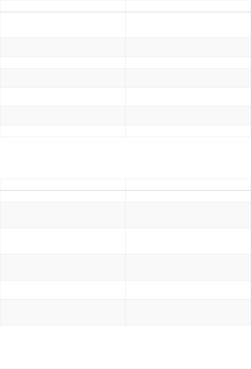
These functions return lists of other values. Further details and examples of lists may be found in
Lists.
Function Description
keys() Returns a list containing the string
representations for all the property names of a
node, relationship, or map.
labels() Returns a list containing the string
representations for all the labels of a node.
nodes() Returns a list containing all the nodes in a path.
range() Returns a list comprising all integer values
within a specified range.
relationships() Returns a list containing all the relationships in
a path.
reverse() Returns a list in which the order of all elements
in the original list have been reversed.
tail() Returns all but the first element in a list.
Mathematical functions - numeric
These functions all operate on numerical expressions only, and will return an error if used on any
other values.
Function Description
abs() Returns the absolute value of a number.
ceil() Returns the smallest floating point number that
is greater than or equal to a number and equal
to a mathematical integer.
floor() Returns the largest floating point number that is
less than or equal to a number and equal to a
mathematical integer.
rand() Returns a random floating point number in the
range from 0 (inclusive) to 1 (exclusive); i.e.
[0,1).
round() Returns the value of a number rounded to the
nearest integer.
sign() Returns the signum of a number: 0 if the
number is 0, -1 for any negative number, and 1
for any positive number.
Mathematical functions - logarithmic
These functions all operate on numerical expressions only, and will return an error if used on any
134

other values.
Function Description
e() Returns the base of the natural logarithm, e.
exp() Returns e^n, where e is the base of the natural
logarithm, and n is the value of the argument
expression.
log() Returns the natural logarithm of a number.
log10() Returns the common logarithm (base 10) of a
number.
sqrt() Returns the square root of a number.
Mathematical functions - trigonometric
These functions all operate on numerical expressions only, and will return an error if used on any
other values.
All trigonometric functions operate on radians, unless otherwise specified.
Function Description
acos() Returns the arccosine of a number in radians.
asin() Returns the arcsine of a number in radians.
atan() Returns the arctangent of a number in radians.
atan2() Returns the arctangent2 of a set of coordinates
in radians.
cos() Returns the cosine of a number.
cot() Returns the cotangent of a number.
degrees() Converts radians to degrees.
pi() Returns the mathematical constant pi.
radians() Converts degrees to radians.
sin() Returns the sine of a number.
tan() Returns the tangent of a number.
String functions
These functions are used to manipulate strings or to create a string representation of another value.
Function Description
left() Returns a string containing the specified
number of leftmost characters of the original
string.
135

Function Description
lTrim() Returns the original string with leading
whitespace removed.
replace() Returns a string in which all occurrences of a
specified string in the original string have been
replaced by another (specified) string.
reverse() Returns a string in which the order of all
characters in the original string have been
reversed.
right() Returns a string containing the specified
number of rightmost characters of the original
string.
rTrim() Returns the original string with trailing
whitespace removed.
split() Returns a list of strings resulting from the
splitting of the original string around matches of
the given delimiter.
substring() Returns a substring of the original string,
beginning with a 0-based index start and length.
toLower() Returns the original string in lowercase.
toString() Converts an integer, float or boolean value to a
string.
toUpper() Returns the original string in uppercase.
trim() Returns the original string with leading and
trailing whitespace removed.
Predicate functions
Predicates are boolean functions that return true or false for a given set of
input. They are most commonly used to filter out subgraphs in the WHERE part of a
query.
Functions:
• exists()
136

name = 'Alice'
age = 38
eyes = 'brown'
name = 'Charlie'
surname = 'Brown'
age = 53
eyes = 'green'
KNOWS
name = 'Bob'
surname = 'Smith'
age = 25
eyes = 'blue'
KNOWS
name = 'Daniel'
age = 54
eyes = 'brown'
KNOWS
array = ['one', 'two', 'three']
name = 'Eskil'
age = 41
eyes = 'blue'
MARRIEDKNOWS
Figure 17. Graph
exists()
exists() returns true if the specified property exists in the node, relationship or map.
Syntax: exists(property)
Returns:
A Boolean.
Arguments:
Name Description
property
A property (in the form 'variable.prop').
Query
MATCH (n)
WHERE exists(n.surname)
RETURN n.name AS name, n.surname AS surname
The names and surnames of all nodes with a surname property are returned.
Table 104. Result
name surname
"Bob" Smith
"Charlie" Brown
2 rows
Scalar functions
Scalar functions return a single value.
137

Functions:
• coalesce()
• endNode()
• head()
• id()
• last()
• length()
• properties()
• size()
• Size of pattern expression
• Size of string
• startNode()
• timestamp()
• toBoolean()
• toFloat()
• toInteger()
• type()
Developer
name = 'Alice'
age = 38
eyes = 'brown'
name = 'Charlie'
age = 53
eyes = 'green'
KNOWS
name = 'Bob'
age = 25
eyes = 'blue'
KNOWS
name = 'Daniel'
age = 54
eyes = 'brown'
KNOWS
array = ['one', 'two', 'three']
name = 'Eskil'
age = 41
eyes = 'blue'
MARRIEDKNOWS
Figure 18. Graph
coalesce()
coalesce() returns the first non-null value in the given list of expressions.
Syntax: coalesce(expression [, expression]*)
Returns:
The type of the value returned will be that of the first non-null expression.
Arguments:
138

Name Description
expression
An expression which may return null.
Considerations:
null will be returned if all the arguments are null.
Query
MATCH (a)
WHERE a.name = 'Alice'
RETURN coalesce(a.hairColor, a.eyes)
Table 105. Result
coalesce(a.hairColor, a.eyes)
"brown"
1 row
endNode()
endNode() returns the end node of a relationship.
Syntax: endNode(relationship)
Returns:
A Node.
Arguments:
Name Description
relationship
An expression that returns a relationship.
Considerations:
endNode(null) returns null.
Query
MATCH (x:Developer)-[r]-()
RETURN endNode(r)
Table 106. Result
139

endNode(r)
Node[2]{name:"Charlie",age:53,eyes:"green"}
Node[1]{name:"Bob",age:25,eyes:"blue"}
2 rows
head()
head() returns the first element in a list.
Syntax: head(list)
Returns:
The type of the value returned will be that of the first element of list.
Arguments:
Name Description
list
An expression that returns a list.
Considerations:
head(null) returns null.
If the first element in list is null, head(list) will return null.
Query
MATCH (a)
WHERE a.name = 'Eskil'
RETURN a.array, head(a.array)
The first element in the list is returned.
Table 107. Result
a.array head(a.array)
["one","two","three"] "one"
1 row
id()
id() returns the id of a relationship or node.
Syntax: id(expression)
Returns:
140

An Integer.
Arguments:
Name Description
expression
An expression that returns a node or a
relationship.
Considerations:
id(null) returns null.
Query
MATCH (a)
RETURN id(a)
The node id for each of the nodes is returned.
Table 108. Result
id(a)
0
1
2
3
4
5 rows
last()
last() returns the last element in a list.
Syntax: last(expression)
Returns:
The type of the value returned will be that of the last element of list.
Arguments:
Name Description
list
An expression that returns a list.
Considerations:
141

last(null) returns null.
If the last element in list is null, last(list) will return null.
Query
MATCH (a)
WHERE a.name = 'Eskil'
RETURN a.array, last(a.array)
The last element in the list is returned.
Table 109. Result
a.array last(a.array)
["one","two","three"] "three"
1 row
length()
length() returns the length of a path.
Syntax: length(path)
Returns:
An Integer.
Arguments:
Name Description
path
An expression that returns a path.
Considerations:
length(null) returns null.
Query
MATCH p = (a)-[]->(b)-[]->(c)
WHERE a.name = 'Alice'
RETURN length(p)
The length of the path p is returned.
Table 110. Result
142

length(p)
2
2
2
3 rows
properties()
properties() returns a map containing all the properties of a node or relationship. If the argument
is already a map, it is returned unchanged.
Syntax: properties(expression)
Returns:
A Map.
Arguments:
Name Description
expression
An expression that returns a node, a
relationship, or a map.
Considerations:
properties(null) returns null.
Query
CREATE (p:Person {name: 'Stefan', city: 'Berlin'})
RETURN properties(p)
Table 111. Result
properties(p)
{name -> "Stefan", city -> "Berlin"}
1 row
Nodes created: 1
Properties set: 2
Labels added: 1
size()
size() returns the number of elements in a list.
Syntax: size(list)
143

Returns:
An Integer.
Arguments:
Name Description
list
An expression that returns a list.
Considerations:
size(null) returns null.
Query
RETURN size(['Alice', 'Bob'])
Table 112. Result
size(['Alice', 'Bob'])
2
1 row
The number of elements in the list is returned.
size() applied to pattern expression
This is the same size() method as described above, but instead of passing in a list directly, a pattern
expression can be provided that can be used in a match query to provide a new set of results. The
size of the result is calculated, not the length of the expression itself.
Syntax: size(pattern expression)
Arguments:
Name Description
pattern expression
A pattern expression that returns a list.
Query
MATCH (a)
WHERE a.name = 'Alice'
RETURN size((a)-[]->()-[]->()) AS fof
Table 113. Result
144

fof
3
1 row
The number of sub-graphs matching the pattern expression is returned.
size() applied to string
size() returns the size of a string value.
Syntax: size(string)
Returns:
An Integer.
Arguments:
Name Description
string
An expression that returns a string value.
Considerations:
size(null) returns null.
Query
MATCH (a)
WHERE size(a.name)> 6
RETURN size(a.name)
Table 114. Result
size(a.name)
7
1 row
The size of the string 'Charlie' is returned.
startNode()
startNode() returns the start node of a relationship.
Syntax: startNode(relationship)
Returns:
145

A Node.
Arguments:
Name Description
relationship
An expression that returns a relationship.
Considerations:
startNode(null) returns null.
Query
MATCH (x:Developer)-[r]-()
RETURN startNode(r)
Table 115. Result
startNode(r)
Node[0]{name:"Alice",age:38,eyes:"brown"}
Node[0]{name:"Alice",age:38,eyes:"brown"}
2 rows
timestamp()
timestamp() returns the difference, measured in milliseconds, between the current time and
midnight, January 1, 1970 UTC.
Syntax: timestamp()
Returns:
An Integer.
Considerations:
timestamp() will return the same value during one entire query, even for long-running queries.
Query
RETURN timestamp()
The time in milliseconds is returned.
Table 116. Result
146

timestamp()
1509846444978
1 row
toBoolean()
toBoolean() converts a string value to a boolean value.
Syntax: toBoolean(expression)
Returns:
A Boolean.
Arguments:
Name Description
expression
An expression that returns a boolean or string
value.
Considerations:
toBoolean(null) returns null.
If expression is a boolean value, it will be returned unchanged.
If the parsing fails, null will be returned.
Query
RETURN toBoolean('TRUE'), toBoolean('not a boolean')
Table 117. Result
toBoolean('TRUE') toBoolean('not a boolean')
true <null>
1 row
toFloat()
toFloat() converts an integer or string value to a floating point number.
Syntax: toFloat(expression)
Returns:
A Float.
147

Arguments:
Name Description
expression
An expression that returns a numeric or string
value.
Considerations:
toFloat(null) returns null.
If expression is a floating point number, it will be returned unchanged.
If the parsing fails, null will be returned.
Query
RETURN toFloat('11.5'), toFloat('not a number')
Table 118. Result
toFloat('11.5') toFloat('not a number')
11.5 <null>
1 row
toInteger()
toInteger() converts a floating point or string value to an integer value.
Syntax: toInteger(expression)
Returns:
An Integer.
Arguments:
Name Description
expression
An expression that returns a numeric or string
value.
Considerations:
toInteger(null) returns null.
If expression is an integer value, it will be returned unchanged.
If the parsing fails, null will be returned.
148

Query
RETURN toInteger('42'), toInteger('not a number')
Table 119. Result
toInteger('42') toInteger('not a number')
42 <null>
1 row
type()
type() returns the string representation of the relationship type.
Syntax: type(relationship)
Returns:
A String.
Arguments:
Name Description
relationship
An expression that returns a relationship.
Considerations:
type(null) returns null.
Query
MATCH (n)-[r]->()
WHERE n.name = 'Alice'
RETURN type(r)
The relationship type of r is returned.
Table 120. Result
type(r)
"KNOWS"
"KNOWS"
2 rows
149

Aggregating functions
To calculate aggregated data, Cypher offers aggregation, analogous to SQL’s GROUP BY.
Aggregating functions take a set of values and calculate an aggregated value over them. Examples
are avg() that calculates the average of multiple numeric values, or min() that finds the smallest
numeric or string value in a set of values. When we say below that an aggregating function
operates on a set of values, we mean these to be the result of the application of the inner expression
(such as n.age) to all the records within the same aggregation group.
Aggregation can be computed over all the matching subgraphs, or it can be further divided by
introducing grouping keys. These are non-aggregate expressions, that are used to group the values
going into the aggregate functions.
Assume we have the following return statement:
RETURN n, count(*)
We have two return expressions: n, and count(*). The first, n, is not an aggregate function, and so it
will be the grouping key. The latter, count(*) is an aggregate expression. The matching subgraphs
will be divided into different buckets, depending on the grouping key. The aggregate function will
then be run on these buckets, calculating an aggregate value per bucket.
To use aggregations to sort the result set, the aggregation must be included in the RETURN to be used
in the ORDER BY.
The DISTINCT operator works in conjunction with aggregation. It is used to make all values unique
before running them through an aggregate function. More information about DISTINCT may be
found here.
Functions:
• avg()
• collect()
• count()
• max()
• min()
• percentileCont()
• percentileDisc()
• stDev()
• stDevP()
• sum()
The following graph is used for the examples below:
150

Person
name = 'A'
age = 13
Person
name = 'B'
age = 33
eyes = 'blue'
KNOWS
Person
name = 'C'
age = 44
eyes = 'blue'
KNOWS
Person
name = 'D'
eyes = 'brown'
KNOWS
Person
name = 'D'
KNOWS KNOWS
Figure 19. Graph
avg()
avg() returns the average of a set of numeric values.
Syntax: avg(expression)
Returns:
Either an Integer or a Float, depending on the values returned by expression and whether or not
the calculation overflows.
Arguments:
Name Description
expression
An expression returning a set of numeric values.
Considerations:
Any null values are excluded from the calculation.
avg(null) returns null.
Query
MATCH (n:Person)
RETURN avg(n.age)
The average of all the values in the property age is returned.
Table 121. Result
avg(n.age)
30.0
1 row
151

collect()
collect() returns a list containing the values returned by an expression. Using this function
aggregates data by amalgamating multiple records or values into a single list.
Syntax: collect(expression)
Returns:
A list containing heterogeneous elements; the types of the elements are determined by the values
returned by expression.
Arguments:
Name Description
expression
An expression returning a set of values.
Considerations:
Any null values are ignored and will not be added to the list.
collect(null) returns an empty list.
Query
MATCH (n:Person)
RETURN collect(n.age)
All the values are collected and returned in a single list.
Table 122. Result
collect(n.age)
[13,33,44]
1 row
count()
count() returns the number of values or records, and appears in two variants:
• count(*) returns the number of matching records, and
• count(expr) returns the number of non-null values returned by an expression.
Syntax: count(expression)
Returns:
An Integer.
152

Arguments:
Name Description
expression
An expression.
Considerations:
count(*) includes records returning null.
count(expr) ignores null values.
count(null) returns 0.
Using count(*) to return the number of nodes
count(*) can be used to return the number of nodes; for example, the number of nodes connected
to some node n.
Query
MATCH (n {name: 'A'})-[]->(x)
RETURN labels(n), n.age, count(*)
The labels and age property of the start node n and the number of nodes related to n are returned.
Table 123. Result
labels(n) n.age count(*)
["Person"] 13 3
1 row
Using count(*) to group and count relationship types
count(*) can be used to group relationship types and return the number.
Query
MATCH (n {name: 'A'})-[r]->()
RETURN type(r), count(*)
The relationship types and their group count are returned.
Table 124. Result
type(r) count(*)
"KNOWS" 3
1 row
153

Using count(expression) to return the number of values
Instead of simply returning the number of records with count(*), it may be more useful to return
the actual number of values returned by an expression.
Query
MATCH (n {name: 'A'})-[]->(x)
RETURN count(x)
The number of nodes connected to the start node is returned.
Table 125. Result
count(x)
3
1 row
Counting non-null values
count(expression) can be used to return the number of non-null values returned by the expression.
Query
MATCH (n:Person)
RETURN count(n.age)
The number of :Person nodes having an age property is returned.
Table 126. Result
count(n.age)
3
1 row
Counting with and without duplicates
In this example we are trying to find all our friends of friends, and count them:
• The first aggregate function, count(DISTINCT friend_of_friend), will only count a
friend_of_friend once, as DISTINCT removes the duplicates.
• The second aggregate function, count(friend_of_friend), will consider the same
friend_of_friend multiple times.
154

Query
MATCH (me:Person)-[]->(friend:Person)-[]->(friend_of_friend:Person)
WHERE me.name = 'A'
RETURN count(DISTINCT friend_of_friend), count(friend_of_friend)
Both B and C know D and thus D will get counted twice when not using DISTINCT.
Table 127. Result
count(DISTINCT friend_of_friend) count(friend_of_friend)
1 2
1 row
max()
max() returns the maximum value in a set of values.
Syntax: max(expression)
Returns:
A property type, or a list, depending on the values returned by expression.
Arguments:
Name Description
expression
An expression returning a set containing any
combination of property types and lists thereof.
Considerations:
Any null values are excluded from the calculation.
In a mixed set, any numeric value is always considered to be higher than any string value, and any
string value is always considered to be higher than any list.
Lists are compared in dictionary order, i.e. list elements are compared pairwise in ascending order
from the start of the list to the end.
max(null) returns null.
Query
UNWIND [1, 'a', NULL, 0.2, 'b', '1', '99'] AS val
RETURN max(val)
The highest of all the values in the mixed set — in this case, the numeric value 1 — is returned. Note
that the (string) value "99", which may appear at first glance to be the highest value in the list, is
155

considered to be a lower value than 1 as the latter is a string.
Table 128. Result
max(val)
1
1 row
Query
UNWIND [[1, 'a', 89],[1, 2]] AS val
RETURN max(val)
The highest of all the lists in the set — in this case, the list [1, 2] — is returned, as the number 2 is
considered to be a higher value than the string "a", even though the list [1, 'a', 89] contains more
elements.
Table 129. Result
max(val)
[1,2]
1 row
Query
MATCH (n:Person)
RETURN max(n.age)
The highest of all the values in the property age is returned.
Table 130. Result
max(n.age)
44
1 row
min()
min() returns the minimum value in a set of values.
Syntax: min(expression)
Returns:
A property type, or a list, depending on the values returned by expression.
Arguments:
156

Name Description
expression
An expression returning a set containing any
combination of property types and lists thereof.
Considerations:
Any null values are excluded from the calculation.
In a mixed set, any string value is always considered to be lower than any numeric value, and any
list is always considered to be lower than any string.
Lists are compared in dictionary order, i.e. list elements are compared pairwise in ascending order
from the start of the list to the end.
min(null) returns null.
Query
UNWIND [1, 'a', NULL, 0.2, 'b', '1', '99'] AS val
RETURN min(val)
The lowest of all the values in the mixed set — in this case, the string value "1" — is returned. Note
that the (numeric) value 0.2, which may appear at first glance to be the lowest value in the list, is
considered to be a higher value than "1" as the latter is a string.
Table 131. Result
min(val)
"1"
1 row
Query
UNWIND ['d',[1, 2],['a', 'c', 23]] AS val
RETURN min(val)
The lowest of all the values in the set — in this case, the list ['a', 'c', 23] — is returned, as (i) the
two lists are considered to be lower values than the string "d", and (ii) the string "a" is considered to
be a lower value than the numerical value 1.
Table 132. Result
min(val)
["a","c",23]
1 row
157

Query
MATCH (n:Person)
RETURN min(n.age)
The lowest of all the values in the property age is returned.
Table 133. Result
min(n.age)
13
1 row
percentileCont()
percentileCont() returns the percentile of the given value over a group, with a percentile from 0.0
to 1.0. It uses a linear interpolation method, calculating a weighted average between two values if
the desired percentile lies between them. For nearest values using a rounding method, see
percentileDisc.
Syntax: percentileCont(expression, percentile)
Returns:
A Float.
Arguments:
Name Description
expression
A numeric expression.
percentile
A numeric value between 0.0 and 1.0
Considerations:
Any null values are excluded from the calculation.
percentileCont(null, percentile) returns null.
Query
MATCH (n:Person)
RETURN percentileCont(n.age, 0.4)
The 40th percentile of the values in the property age is returned, calculated with a weighted
average. In this case, 0.4 is the median, or 40th percentile.
Table 134. Result
158

percentileCont(n.age, 0.4)
29.0
1 row
percentileDisc()
percentileDisc() returns the percentile of the given value over a group, with a percentile from 0.0
to 1.0. It uses a rounding method and calculates the nearest value to the percentile. For interpolated
values, see percentileCont.
Syntax: percentileDisc(expression, percentile)
Returns:
Either an Integer or a Float, depending on the values returned by expression and whether or not
the calculation overflows.
Arguments:
Name Description
expression
A numeric expression.
percentile
A numeric value between 0.0 and 1.0
Considerations:
Any null values are excluded from the calculation.
percentileDisc(null, percentile) returns null.
Query
MATCH (n:Person)
RETURN percentileDisc(n.age, 0.5)
The 50th percentile of the values in the property age is returned.
Table 135. Result
percentileDisc(n.age, 0.5)
33
1 row
stDev()
stDev() returns the standard deviation for the given value over a group. It uses a standard two-pass
method, with N - 1 as the denominator, and should be used when taking a sample of the population
159

for an unbiased estimate. When the standard variation of the entire population is being calculated,
stdDevP should be used.
Syntax: stDev(expression)
Returns:
A Float.
Arguments:
Name Description
expression
A numeric expression.
Considerations:
Any null values are excluded from the calculation.
stDev(null) returns 0.
Query
MATCH (n)
WHERE n.name IN ['A', 'B', 'C']
RETURN stDev(n.age)
The standard deviation of the values in the property age is returned.
Table 136. Result
stDev(n.age)
15.716233645501712
1 row
stDevP()
stDevP() returns the standard deviation for the given value over a group. It uses a standard two-
pass method, with N as the denominator, and should be used when calculating the standard
deviation for an entire population. When the standard variation of only a sample of the population
is being calculated, stDev should be used.
Syntax: stDevP(expression)
Returns:
A Float.
Arguments:
160

Name Description
expression
A numeric expression.
Considerations:
Any null values are excluded from the calculation.
stDevP(null) returns 0.
Query
MATCH (n)
WHERE n.name IN ['A', 'B', 'C']
RETURN stDevP(n.age)
The population standard deviation of the values in the property age is returned.
Table 137. Result
stDevP(n.age)
12.832251036613439
1 row
sum()
sum() returns the sum of a set of numeric values.
Syntax: sum(expression)
Returns:
Either an Integer or a Float, depending on the values returned by expression.
Arguments:
Name Description
expression
An expression returning a set of numeric values.
Considerations:
Any null values are excluded from the calculation.
sum(null) returns 0.
161

Query
MATCH (n:Person)
RETURN sum(n.age)
The sum of all the values in the property age is returned.
Table 138. Result
sum(n.age)
90
1 row
List functions
List functions return lists of things — nodes in a path, and so on.
Further details and examples of lists may be found in Lists and List operators.
Functions:
• keys()
• labels()
• nodes()
• range()
• relationships()
• reverse()
• tail()
Person, Developer
name = 'Alice'
age = 38
eyes = 'brown'
name = 'Charlie'
age = 53
eyes = 'green'
KNOWS
name = 'Bob'
age = 25
eyes = 'blue'
KNOWS
name = 'Daniel'
age = 54
eyes = 'brown'
KNOWS
array = ['one', 'two', 'three']
name = 'Eskil'
age = 41
eyes = 'blue'
MARRIEDKNOWS
Figure 20. Graph
keys()
keys returns a list containing the string representations for all the property names of a node,
162

relationship, or map.
Syntax: keys(expression)
Returns:
A list containing String elements.
Arguments:
Name Description
expression
An expression that returns a node, a
relationship, or a map.
Considerations:
keys(null) returns null.
Query
MATCH (a)
WHERE a.name = 'Alice'
RETURN keys(a)
A list containing the names of all the properties on the node bound to a is returned.
Table 139. Result
keys(a)
["name","age","eyes"]
1 row
labels()
labels returns a list containing the string representations for all the labels of a node.
Syntax: labels(node)
Returns:
A list containing String elements.
Arguments:
Name Description
node
An expression that returns a single node.
163

Considerations:
labels(null) returns null.
Query
MATCH (a)
WHERE a.name = 'Alice'
RETURN labels(a)
A list containing all the labels of the node bound to a is returned.
Table 140. Result
labels(a)
["Person","Developer"]
1 row
nodes()
nodes() returns a list containing all the nodes in a path.
Syntax: nodes(path)
Returns:
A list containing Node elements.
Arguments:
Name Description
path
An expression that returns a path.
Considerations:
nodes(null) returns null.
Query
MATCH p = (a)-[]->(b)-[]->(c)
WHERE a.name = 'Alice' AND c.name = 'Eskil'
RETURN nodes(p)
A list containing all the nodes in the path p is returned.
Table 141. Result
164

nodes(p)
[Node[0]{name:"Alice",age:38,eyes:"brown"},Node[1]{name:"Bob",age:25,eyes:"blue"},Node[4]{arra
y:["one","two","three"],name:"Eskil",age:41,eyes:"blue"}]
1 row
range()
range() returns a list comprising all integer values within a range bounded by a start value start
and end value end, where the difference step between any two consecutive values is constant; i.e.
an arithmetic progression. The range is inclusive, and the arithmetic progression will therefore
always contain start and — depending on the values of start, step and end — end.
Syntax: range(start, end [, step])
Returns:
A list of Integer elements.
Arguments:
Name Description
start
An expression that returns an integer value.
end
An expression that returns an integer value.
step
A numeric expression defining the difference
between any two consecutive values, with a
default of 1.
Query
RETURN range(0, 10), range(2, 18, 3)
Two lists of numbers in the given ranges are returned.
Table 142. Result
range(0, 10) range(2, 18, 3)
[0,1,2,3,4,5,6,7,8,9,10] [2,5,8,11,14,17]
1 row
relationships()
relationships() returns a list containing all the relationships in a path.
Syntax: relationships(path)
Returns:
165

A list containing Relationship elements.
Arguments:
Name Description
path
An expression that returns a path.
Considerations:
relationships(null) returns null.
Query
MATCH p = (a)-[]->(b)-[]->(c)
WHERE a.name = 'Alice' AND c.name = 'Eskil'
RETURN relationships(p)
A list containing all the relationships in the path p is returned.
Table 143. Result
relationships(p)
[:KNOWS[0]{},:MARRIED[4]{}]
1 row
reverse()
reverse() returns a list in which the order of all elements in the original list have been reversed.
Syntax: reverse(original)
Returns:
A list containing homogeneous or heterogeneous elements; the types of the elements are
determined by the elements within original.
Arguments:
Name Description
original
An expression that returns a list.
Considerations:
Any null element in original is preserved.
166

Query
WITH [4923, 'abc', 521, NULL, 487] AS ids
RETURN reverse(ids)
Table 144. Result
reverse(ids)
[487,<null>,521,"abc",4923]
1 row
tail()
tail() returns a list l
result
containing all the elements, excluding the first one, from a list list.
Syntax: tail(list)
Returns:
A list containing heterogeneous elements; the types of the elements are determined by the
elements in list.
Arguments:
Name Description
list
An expression that returns a list.
Query
MATCH (a)
WHERE a.name = 'Eskil'
RETURN a.array, tail(a.array)
The property named array and a list comprising all but the first element of the array property are
returned.
Table 145. Result
a.array tail(a.array)
["one","two","three"] ["two","three"]
1 row
Mathematical functions - numeric
These functions all operate on numeric expressions only, and will return
167

an error if used on any other values. See also Mathematical operators.
Functions:
• abs()
• ceil()
• floor()
• rand()
• round()
• sign()
The following graph is used for the examples below:
A
name = 'Alice'
age = 38
eyes = 'brown'
C
name = 'Charlie'
age = 53
eyes = 'green'
KNOWS
B
name = 'Bob'
age = 25
eyes = 'blue'
KNOWS
D
name = 'Daniel'
age = 54
eyes = 'brown'
KNOWS
E
array = ['one', 'two', 'three']
name = 'Eskil'
age = 41
eyes = 'blue'
MARRIEDKNOWS
Figure 21. Graph
abs()
abs() returns the absolute value of the given number.
Syntax: abs(expression)
Returns:
The type of the value returned will be that of expression.
Arguments:
Name Description
expression
A numeric expression.
Considerations:
abs(null) returns null.
If expression is negative, -(expression) (i.e. the negation of expression) is returned.
168

Query
MATCH (a), (e)
WHERE a.name = 'Alice' AND e.name = 'Eskil'
RETURN a.age, e.age, abs(a.age - e.age)
The absolute value of the age difference is returned.
Table 146. Result
a.age e.age abs(a.age - e.age)
38 41 3
1 row
ceil()
ceil() returns the smallest floating point number that is greater than or equal to the given number
and equal to a mathematical integer.
Syntax: ceil(expression)
Returns:
A Float.
Arguments:
Name Description
expression
A numeric expression.
Considerations:
ceil(null) returns null.
Query
RETURN ceil(0.1)
The ceil of 0.1 is returned.
Table 147. Result
ceil(0.1)
1.0
1 row
169

floor()
floor() returns the largest floating point number that is less than or equal to the given number and
equal to a mathematical integer.
Syntax: floor(expression)
Returns:
A Float.
Arguments:
Name Description
expression
A numeric expression.
Considerations:
floor(null) returns null.
Query
RETURN floor(0.9)
The floor of 0.9 is returned.
Table 148. Result
floor(0.9)
0.0
1 row
rand()
rand() returns a random floating point number in the range from 0 (inclusive) to 1 (exclusive); i.e.
[0,1). The numbers returned follow an approximate uniform distribution.
Syntax: rand()
Returns:
A Float.
Query
RETURN rand()
170

A random number is returned.
Table 149. Result
rand()
0.3586784748902053
1 row
round()
round() returns the value of the given number rounded to the nearest integer.
Syntax: round(expression)
Returns:
A Float.
Arguments:
Name Description
expression
A numeric expression.
Considerations:
round(null) returns null.
Query
RETURN round(3.141592)
3.0 is returned.
Table 150. Result
round(3.141592)
3.0
1 row
sign()
sign() returns the signum of the given number: 0 if the number is 0, -1 for any negative number,
and 1 for any positive number.
Syntax: sign(expression)
Returns:
171

An Integer.
Arguments:
Name Description
expression
A numeric expression.
Considerations:
sign(null) returns null.
Query
RETURN sign(-17), sign(0.1)
The signs of -17 and 0.1 are returned.
Table 151. Result
sign(-17) sign(0.1)
-1 1
1 row
Mathematical functions - logarithmic
These functions all operate on numeric expressions only, and will return
an error if used on any other values. See also Mathematical operators.
Functions:
• e()
• exp()
• log()
• log10()
• sqrt()
e()
e() returns the base of the natural logarithm, e.
Syntax: e()
Returns:
172

A Float.
Query
RETURN e()
The base of the natural logarithm, e, is returned.
Table 152. Result
e()
2.718281828459045
1 row
exp()
exp() returns e^n, where e is the base of the natural logarithm, and n is the value of the argument
expression.
Syntax: e(expression)
Returns:
A Float.
Arguments:
Name Description
expression
A numeric expression.
Considerations:
exp(null) returns null.
Query
RETURN exp(2)
e to the power of 2 is returned.
Table 153. Result
exp(2)
7.38905609893065
1 row
173

log()
log() returns the natural logarithm of a number.
Syntax: log(expression)
Returns:
A Float.
Arguments:
Name Description
expression
A numeric expression.
Considerations:
log(null) returns null.
log(0) returns null.
Query
RETURN log(27)
The natural logarithm of 27 is returned.
Table 154. Result
log(27)
3.295836866004329
1 row
log10()
log10() returns the common logarithm (base 10) of a number.
Syntax: log10(expression)
Returns:
A Float.
Arguments:
Name Description
expression
A numeric expression.
174

Considerations:
log10(null) returns null.
log10(0) returns null.
Query
RETURN log10(27)
The common logarithm of 27 is returned.
Table 155. Result
log10(27)
1.4313637641589874
1 row
sqrt()
sqrt() returns the square root of a number.
Syntax: sqrt(expression)
Returns:
A Float.
Arguments:
Name Description
expression
A numeric expression.
Considerations:
sqrt(null) returns null.
sqrt(<any negative number>) returns null
Query
RETURN sqrt(256)
The square root of 256 is returned.
Table 156. Result
175

sqrt(256)
16.0
1 row
Mathematical functions - trigonometric
These functions all operate on numeric expressions only, and will return
an error if used on any other values. See also Mathematical operators.
Functions:
• acos()
• asin()
• atan()
• atan2()
• cos()
• cot()
• degrees()
• pi()
• radians()
• sin()
• tan()
acos()
acos() returns the arccosine of a number in radians.
Syntax: acos(expression)
Returns:
A Float.
Arguments:
Name Description
expression
A numeric expression that represents the angle
in radians.
Considerations:
acos(null) returns null.
176

If (expression < -1) or (expression > 1), then (acos(expression)) returns null.
Query
RETURN acos(0.5)
The arccosine of 0.5 is returned.
Table 157. Result
acos(0.5)
1.0471975511965979
1 row
asin()
asin() returns the arcsine of a number in radians.
Syntax: asin(expression)
Returns:
A Float.
Arguments:
Name Description
expression
A numeric expression that represents the angle
in radians.
Considerations:
asin(null) returns null.
If (expression < -1) or (expression > 1), then (asin(expression)) returns null.
Query
RETURN asin(0.5)
The arcsine of 0.5 is returned.
Table 158. Result
asin(0.5)
0.5235987755982989
1 row
177

atan()
atan() returns the arctangent of a number in radians.
Syntax: atan(expression)
Returns:
A Float.
Arguments:
Name Description
expression
A numeric expression that represents the angle
in radians.
Considerations:
atan(null) returns null.
Query
RETURN atan(0.5)
The arctangent of 0.5 is returned.
Table 159. Result
atan(0.5)
0.4636476090008061
1 row
atan2()
atan2() returns the arctangent2 of a set of coordinates in radians.
Syntax: atan2(expression1, expression2)
Returns:
A Float.
Arguments:
Name Description
expression1
A numeric expression for y that represents the
angle in radians.
178

Name Description
expression2
A numeric expression for x that represents the
angle in radians.
Considerations:
atan2(null, null), atan2(null, expression2) and atan(expression1, null) all return null.
Query
RETURN atan2(0.5, 0.6)
The arctangent2 of 0.5 and 0.6 is returned.
Table 160. Result
atan2(0.5, 0.6)
0.6947382761967033
1 row
cos()
cos() returns the cosine of a number.
Syntax: cos(expression)
Returns:
A Float.
Arguments:
Name Description
expression
A numeric expression that represents the angle
in radians.
Considerations:
cos(null) returns null.
Query
RETURN cos(0.5)
The cosine of 0.5 is returned.
179

Table 161. Result
cos(0.5)
0.8775825618903728
1 row
cot()
cot() returns the cotangent of a number.
Syntax: cot(expression)
Returns:
A Float.
Arguments:
Name Description
expression
A numeric expression that represents the angle
in radians.
Considerations:
cot(null) returns null.
cot(0) returns null.
Query
RETURN cot(0.5)
The cotangent of 0.5 is returned.
Table 162. Result
cot(0.5)
1.830487721712452
1 row
degrees()
degrees() converts radians to degrees.
Syntax: degrees(expression)
Returns:
180

A Float.
Arguments:
Name Description
expression
A numeric expression that represents the angle
in radians.
Considerations:
degrees(null) returns null.
Query
RETURN degrees(3.14159)
The number of degrees in something close to pi is returned.
Table 163. Result
degrees(3.14159)
179.99984796050427
1 row
pi()
pi() returns the mathematical constant pi.
Syntax: pi()
Returns:
A Float.
Query
RETURN pi()
The constant pi is returned.
Table 164. Result
pi()
3.141592653589793
1 row
181

radians()
radians() converts degrees to radians.
Syntax: radians(expression)
Returns:
A Float.
Arguments:
Name Description
expression
A numeric expression that represents the angle
in degrees.
Considerations:
radians(null) returns null.
Query
RETURN radians(180)
The number of radians in 180 degrees is returned (pi).
Table 165. Result
radians(180)
3.141592653589793
1 row
sin()
sin() returns the sine of a number.
Syntax: sin(expression)
Returns:
A Float.
Arguments:
Name Description
expression
A numeric expression that represents the angle
in radians.
182

Considerations:
sin(null) returns null.
Query
RETURN sin(0.5)
The sine of 0.5 is returned.
Table 166. Result
sin(0.5)
0.479425538604203
1 row
tan()
tan() returns the tangent of a number.
Syntax: tan(expression)
Returns:
A Float.
Arguments:
Name Description
expression
A numeric expression that represents the angle
in radians.
Considerations:
tan(null) returns null.
Query
RETURN tan(0.5)
The tangent of 0.5 is returned.
Table 167. Result
tan(0.5)
0.5463024898437905
1 row
183

String functions
These functions all operate on string expressions only, and will return an
error if used on any other values. The exception to this rule is toString(), which
also accepts numbers and booleans.
See also String operators.
Functions:
• left()
• lTrim()
• replace()
• reverse()
• right()
• rTrim()
• split()
• substring()
• toLower()
• toString()
• toUpper()
• trim()
left()
left() returns a string containing the specified number of leftmost characters of the original string.
Syntax: left(original, length)
Returns:
A String.
Arguments:
Name Description
original
An expression that returns a string.
n
An expression that returns a positive integer.
Considerations:
left(null, length) and left(null, null) both return null
184

left(original, null) will raise an error.
If length is not a positive integer, an error is raised.
If length exceeds the size of original, original is returned.
Query
RETURN left('hello', 3)
Table 168. Result
left('hello', 3)
"hel"
1 row
ltrim()
lTrim() returns the original string with leading whitespace removed.
Syntax: lTrim(original)
Returns:
A String.
Arguments:
Name Description
original
An expression that returns a string.
Considerations:
lTrim(null) returns null
Query
RETURN lTrim(' hello')
Table 169. Result
lTrim(' hello')
"hello"
1 row
185

replace()
replace() returns a string in which all occurrences of a specified string in the original string have
been replaced by another (specified) string.
Syntax: replace(original, search, replace)
Returns:
A String.
Arguments:
Name Description
original
An expression that returns a string.
search
An expression that specifies the string to be
replaced in original.
replace
An expression that specifies the replacement
string.
Considerations:
If any argument is null, null will be returned.
If search is not found in original, original will be returned.
Query
RETURN replace("hello", "l", "w")
Table 170. Result
replace("hello", "l", "w")
"hewwo"
1 row
reverse()
reverse() returns a string in which the order of all characters in the original string have been
reversed.
Syntax: reverse(original)
Returns:
A String.
186

Arguments:
Name Description
original
An expression that returns a string.
Considerations:
reverse(null) returns null.
Query
RETURN reverse('anagram')
Table 171. Result
reverse('anagram')
"margana"
1 row
right()
right() returns a string containing the specified number of rightmost characters of the original
string.
Syntax: right(original, length)
Returns:
A String.
Arguments:
Name Description
original
An expression that returns a string.
n
An expression that returns a positive integer.
Considerations:
right(null, length) and right(null, null) both return null
right(original, null) will raise an error.
If length is not a positive integer, an error is raised.
If length exceeds the size of original, original is returned.
187

Query
RETURN right('hello', 3)
Table 172. Result
right('hello', 3)
"llo"
1 row
rtrim()
rTrim() returns the original string with trailing whitespace removed.
Syntax: rTrim(original)
Returns:
A String.
Arguments:
Name Description
original
An expression that returns a string.
Considerations:
rTrim(null) returns null
Query
RETURN rTrim('hello ')
Table 173. Result
rTrim('hello ')
"hello"
1 row
split()
split() returns a list of strings resulting from the splitting of the original string around matches of
the given delimiter.
Syntax: split(original, splitDelimiter)
Returns:
188

A list of Strings.
Arguments:
Name Description
original
An expression that returns a string.
splitDelimiter
The string with which to split original.
Considerations:
split(null, splitDelimiter) and split(original, null) both return null
Query
RETURN split('one,two', ',')
Table 174. Result
split('one,two', ',')
["one","two"]
1 row
substring()
substring() returns a substring of the original string, beginning with a 0-based index start and
length.
Syntax: substring(original, start [, length])
Returns:
A String.
Arguments:
Name Description
original
An expression that returns a string.
start
An expression that returns a positive integer,
denoting the position at which the substring will
begin.
length
An expression that returns a positive integer,
denoting how many characters of original will
be returned.
Considerations:
189

start uses a zero-based index.
If length is omitted, the function returns the substring starting at the position given by start and
extending to the end of original.
If original is null, null is returned.
If either start or length is null or a negative integer, an error is raised.
If start is 0, the substring will start at the beginning of original.
If length is 0, the empty string will be returned.
Query
RETURN substring('hello', 1, 3), substring('hello', 2)
Table 175. Result
substring('hello', 1, 3) substring('hello', 2)
"ell" "llo"
1 row
toLower()
toLower() returns the original string in lowercase.
Syntax: toLower(original)
Returns:
A String.
Arguments:
Name Description
original
An expression that returns a string.
Considerations:
toLower(null) returns null
Query
RETURN toLower('HELLO')
Table 176. Result
190

toLower('HELLO')
"hello"
1 row
toString()
toString() converts an integer, float or boolean value to a string.
Syntax: toString(expression)
Returns:
A String.
Arguments:
Name Description
expression
An expression that returns a number, a boolean,
or a string.
Considerations:
toString(null) returns null
If expression is a string, it will be returned unchanged.
Query
RETURN toString(11.5), toString('already a string'), toString(TRUE )
Table 177. Result
toString(11.5) toString('already a string') toString(true)
"11.5" "already a string" "true"
1 row
toUpper()
toUpper() returns the original string in uppercase.
Syntax: toUpper(original)
Returns:
A String.
Arguments:
191

Name Description
original
An expression that returns a string.
Considerations:
toUpper(null) returns null
Query
RETURN toUpper('hello')
Table 178. Result
toUpper('hello')
"HELLO"
1 row
trim()
trim() returns the original string with leading and trailing whitespace removed.
Syntax: trim(original)
Returns:
A String.
Arguments:
Name Description
original
An expression that returns a string.
Considerations:
trim(null) returns null
Query
RETURN trim(' hello ')
Table 179. Result
trim(' hello ')
"hello"
1 row
192

User-defined functions
User-defined functions are called in the same way as any other Cypher function. A user-defined
function must return values within the Cypher type system.
This example shows how to invoke a user-defined function called join from Cypher.
Call a user-defined function
This calls the user-defined function org.opencypher.procedure.example.join().
Query
MATCH (n:Member)
RETURN org.opencypher.function.example.join(collect(n.name)) AS members
Result
+--------------------------+
| members |
+--------------------------+
| "John,Paul,George,Ringo" |
+--------------------------+
1 row
User-defined aggregation functions
User-defined aggregation functions are called in the same way as any other Cypher function. A
user-defined aggregating function must return values within the Cypher type system.
This example shows how to invoke a user-defined aggregation function called longestString from
Cypher.
Call a user-defined aggregation function
This calls the user-defined function org.opencypher.procedure.example.longestString().
Query
MATCH (n:Member)
RETURN org.opencypher.function.example.longestString(n.name) AS member
193

Result
+----------+
| member |
+----------+
| "George" |
+----------+
1 row
194

Comments
Comments may be added to queries. Single line — or inline — comments begin with //, and multi-
line comments are delimited by /* and */.
Examples:
MATCH (n) RETURN n //This is an end of line comment
MATCH (n)
//This is a single line comment
RETURN n
MATCH (n) WHERE n.property = '//This is NOT a comment' RETURN n
/* The following comment
spans more than
one line */
MATCH (n)
RETURN n
195

Compatibility and versioning
It may sometimes be necessary to use a previous version of Cypher when running a query.
For example, assume that the semantics of an operator X is altered in Cypher 10, but that in a
particular scenario, it is absolutely necessary to use the semantics of X as defined in Cypher 9. In
cases like these, it is possible to specify, at a query level, which version of Cypher to use.
By starting the Cypher query string with CYPHER <num>, where <num> is one of the standard Cypher
versions (as of this document, only 9), the following query would be interpreted under the
semantics as specified for that version.
This example shows how to specify, for the given query, that the semantics as defined in Cypher 9
are used (assuming the current version is 10 or higher):
Query
CYPHER 9
MATCH (a)-[]->(b)
RETURN a, b
196

Reserved keywords
Historically, Cypher has liberally allowed any word to be used as an identifier, relying on context to
disambiguate between possible uses of a particular word. As Cypher matures towards becoming a
standard language, however, a more generic model that aligns with users' expectations from the
world of programming languages is preferable, and a grammar with clearer distinctions between
identifiers and keywords is a step in that direction. Moreover, queries that are hard to read would
be more difficult to write.
We provide here a listing of reserved words, grouped by the categories from which they are drawn,
all of which have a special meaning in Cypher. In addition to this, we list a number of words that
are reserved for future use. These reserved words are not permitted to be used as identifiers in the
following contexts:
• Variables
• Function names
• Parameters
By escaping any of the reserved words (encapsulating in backticks `), they would be valid as
identifiers in the above contexts.
Clauses
• CREATE
• DELETE
• DETACH
• EXISTS
• MATCH
• MERGE
• OPTIONAL
• REMOVE
• RETURN
• SET
• UNION
• UNWIND
• WITH
Subclauses
• LIMIT
• ORDER
197

• SKIP
• WHERE
Modifiers
• ASC
• ASCENDING
• BY
• DESC
• DESCENDING
• ON
Expressions
• ALL
• CASE
• ELSE
• END
• THEN
• WHEN
Operators
• AND
• AS
• CONTAINS
• DISTINCT
• ENDS
• IN
• IS
• NOT
• OR
• STARTS
• XOR
Literals
• false
198

• null
• true
Reserved for future use
• ADD
• CONSTRAINT
• DO
• DROP
• FOR
• MANDATORY
• OF
• REQUIRE
• SCALAR
• UNIQUE
199

Glossary of keywords
This section comprises a glossary of all the keywords — grouped by
category and thence ordered lexicographically — in the Cypher query language.
• Clauses
• Operators
• Functions
• Expressions
• Cypher query versioning
Clauses
Clause Category Description
CALL […YIELD] Reading/Writing Invoke a procedure deployed in
the database.
CREATE Writing Create nodes and relationships.
DELETE Writing Delete graph elements — nodes,
relationships or paths. Any
node to be deleted must also
have all associated
relationships explicitly deleted.
DETACH DELETE Writing Delete a node or set of nodes.
All associated relationships will
automatically be deleted.
LIMIT Reading sub-clause A sub-clause used to constrain
the number of records in the
output.
MATCH Reading Specify the patterns to search
for in the database.
MANDATORY MATCH Reading Specify the patterns to search
for in the database, and fail if
no match is found.
MERGE Reading/Writing Ensures that a pattern exists in
the graph. Either the pattern
already exists, or it needs to be
created.
OPTIONAL MATCH Reading Specify the patterns to search
for in the database while using
nulls for missing parts of the
pattern.
200

Clause Category Description
ORDER BY [ASC[ENDING] |
DESC[ENDING]]
Reading sub-clause A sub-clause following RETURN or
WITH, specifying that the output
should be sorted in either
ascending (the default) or
descending order.
REMOVE Writing Remove properties and labels
from nodes and relationships.
RETURN … [AS] Projecting Defines what to include in the
query result set.
SET Writing Update labels on nodes and
properties on nodes and
relationships.
SKIP Reading/Writing A sub-clause defining from
which record to start including
the records in the output.
UNION Set operations Combines the result of multiple
queries. Duplicates are
removed.
UNION ALL Set operations Combines the result of multiple
queries. Duplicates are
retained.
UNWIND … [AS] Projecting Expands a list into a sequence
of records.
WITH … [AS] Projecting Allows query parts to be
chained together, piping the
results from one to be used as
starting points or criteria in the
next.
WHERE Reading sub-clause A sub-clause used to add
constraints to the patterns in a
MATCH or OPTIONAL MATCH clause,
or to filter the results of a WITH
clause.
Operators
Operator Category Description
% Mathematical Modulo division
* Mathematical Multiplication
+ Mathematical Addition
+ String Concatenation
201

Operator Category Description
+ List Concatenation
- Mathematical Subtraction or unary minus
. General Property access
/ Mathematical Division
< Comparison Less than
<= Comparison Less than or equal to
<> Comparison Inequality
= Comparison Equality
> Comparison Greater than
>= Comparison Greater than or equal to
AND Boolean Conjunction
CONTAINS String comparison Case-sensitive inclusion search
DISTINCT General Duplicate removal
ENDS WITH String comparison Case-sensitive suffix search
IN List List element existence check
IS NOT NULL Comparison Non-null check
IS NULL Comparison null check
NOT Boolean Negation
OR Boolean Disjunction
STARTS WITH String comparison Case-sensitive prefix search
XOR Boolean Exclusive disjunction
[] General Subscript (dynamic property
access)
[] List Subscript (accessing element(s)
in a list)
^ Mathematical Exponentiation
Functions
Function Category Description
abs() Numeric Returns the absolute value of a
number.
202

Function Category Description
acos() Trigonometric Returns the arccosine of a
number in radians.
asin() Trigonometric Returns the arcsine of a
number in radians.
atan() Trigonometric Returns the arctangent of a
number in radians.
atan2() Trigonometric Returns the arctangent2 of a set
of coordinates in radians.
avg() Aggregating Returns the average of a set of
values.
ceil() Numeric Returns the smallest floating
point number that is greater
than or equal to a number and
equal to a mathematical
integer.
coalesce() Scalar Returns the first non-null value
in a list of expressions.
collect() Aggregating Returns a list containing the
values returned by an
expression.
cos() Trigonometric Returns the cosine of a number.
cot() Trigonometric Returns the cotangent of a
number.
count() Aggregating Returns the number of values
or records.
degrees() Trigonometric Converts radians to degrees.
e() Logarithmic Returns the base of the natural
logarithm, e.
endNode() Scalar Returns the end node of a
relationship.
exists() Predicate Returns true if a match for the
pattern exists in the graph, or if
the specified property exists in
the node, relationship or map.
exp() Logarithmic Returns e^n, where e is the base
of the natural logarithm, and n
is the value of the argument
expression.
203

Function Category Description
floor() Numeric Returns the largest floating
point number that is less than
or equal to a number and equal
to a mathematical integer.
head() Scalar Returns the first element in a
list.
id() Scalar Returns the id of a relationship
or node.
keys() List Returns a list containing the
string representations for all
the property names of a node,
relationship, or map.
labels() List Returns a list containing the
string representations for all
the labels of a node.
last() Scalar Returns the last element in a
list.
left() String Returns a string containing the
specified number of leftmost
characters of the original string.
length() Scalar Returns the length of a path.
log() Logarithmic Returns the natural logarithm
of a number.
log10() Logarithmic Returns the common logarithm
(base 10) of a number.
lTrim() String Returns the original string with
leading whitespace removed.
max() Aggregating Returns the maximum value in
a set of values.
min() Aggregating Returns the minimum value in
a set of values.
nodes() List Returns a list containing all the
nodes in a path.
percentileCont() Aggregating Returns the percentile of the
given value over a group using
linear interpolation.
percentileDisc() Aggregating Returns the nearest value to the
given percentile over a group
using a rounding method.
204

Function Category Description
pi() Trigonometric Returns the mathematical
constant pi.
properties() Scalar Returns a map containing all
the properties of a node or
relationship.
radians() Trigonometric Converts degrees to radians.
rand() Numeric Returns a random floating point
number in the range from 0
(inclusive) to 1 (exclusive); i.e.
[0, 1).
range() List Returns a list comprising all
integer values within a
specified range.
relationships() List Returns a list containing all the
relationships in a path.
replace() String Returns a string in which all
occurrences of a specified
string in the original string
have been replaced by another
(specified) string.
reverse() List Returns a list in which the
order of all elements in the
original list have been reversed.
reverse() String Returns a string in which the
order of all characters in the
original string have been
reversed.
right() String Returns a string containing the
specified number of rightmost
characters of the original string.
round() Numeric Returns the value of a number
rounded to the nearest integer.
rTrim() String Returns the original string with
trailing whitespace removed.
sign() Numeric Returns the signum of a
number: 0 if the number is 0, -1
for any negative number, and 1
for any positive number.
sin() Trigonometric Returns the sine of a number.
size() Scalar Returns the number of items in
a list.
205

Function Category Description
size() applied to pattern
expression
Scalar Returns the number of sub-
graphs matching the pattern
expression.
size() applied to string Scalar Returns the size of a string.
split() String Returns a list of strings
resulting from the splitting of
the original string around
matches of the given delimiter.
sqrt() Logarithmic Returns the square root of a
number.
startNode() Scalar Returns the start node of a
relationship.
stDev() Aggregating Returns the standard deviation
for the given value over a group
for a sample of a population.
stDevP() Aggregating Returns the standard deviation
for the given value over a group
for an entire population.
substring() String Returns a substring of the
original string, beginning with
a 0-based index start and
length.
sum() Aggregating Returns the sum of a set of
numeric values.
tail() List Returns all but the first element
in a list.
tan() Trigonometric Returns the tangent of a
number.
timestamp() Scalar Returns the difference,
measured in milliseconds,
between the current time and
midnight, January 1, 1970 UTC.
toBoolean() Scalar Converts a string value to a
boolean value.
toFloat() Scalar Converts an integer or string
value to a floating point
number.
toInteger() Scalar Converts a floating point or
string value to an integer value.
toLower() String Returns the original string in
lowercase.
206

Function Category Description
toString() String Converts an integer, float or
boolean value to a string.
toUpper() String Returns the original string in
uppercase.
trim() String Returns the original string with
leading and trailing whitespace
removed.
type() Scalar Returns the string
representation of the
relationship type.
Expressions
Name Description
CASE Expression A generic conditional expression, similar to
if/else statements available in other languages.
Cypher query versioning
Name Type Description
CYPHER $version query Version This will force 'query' to use
Cypher $version.
License
Apache License, Version 2.0, January 2004
TERMS AND CONDITIONS FOR USE, REPRODUCTION, AND DISTRIBUTION
1. Definitions.
"License" shall mean the terms and conditions for use, reproduction,
and distribution as defined by Sections 1 through 9 of this document.
"Licensor" shall mean the copyright owner or entity authorized by
the copyright owner that is granting the License.
207

"Legal Entity" shall mean the union of the acting entity and all
other entities that control, are controlled by, or are under common
control with that entity. For the purposes of this definition,
"control" means (i) the power, direct or indirect, to cause the
direction or management of such entity, whether by contract or
otherwise, or (ii) ownership of fifty percent (50%) or more of the
outstanding shares, or (iii) beneficial ownership of such entity.
"You" (or "Your") shall mean an individual or Legal Entity
exercising permissions granted by this License.
"Source" form shall mean the preferred form for making modifications,
including but not limited to software source code, documentation
source, and configuration files.
"Object" form shall mean any form resulting from mechanical
transformation or translation of a Source form, including but
not limited to compiled object code, generated documentation,
and conversions to other media types.
"Work" shall mean the work of authorship, whether in Source or
Object form, made available under the License, as indicated by a
copyright notice that is included in or attached to the work
(an example is provided in the Appendix below).
"Derivative Works" shall mean any work, whether in Source or Object
form, that is based on (or derived from) the Work and for which the
editorial revisions, annotations, elaborations, or other modifications
represent, as a whole, an original work of authorship. For the purposes
of this License, Derivative Works shall not include works that remain
separable from, or merely link (or bind by name) to the interfaces of,
the Work and Derivative Works thereof.
208

"Contribution" shall mean any work of authorship, including
the original version of the Work and any modifications or additions
to that Work or Derivative Works thereof, that is intentionally
submitted to Licensor for inclusion in the Work by the copyright owner
or by an individual or Legal Entity authorized to submit on behalf of
the copyright owner. For the purposes of this definition, "submitted"
means any form of electronic, verbal, or written communication sent
to the Licensor or its representatives, including but not limited to
communication on electronic mailing lists, source code control systems,
and issue tracking systems that are managed by, or on behalf of, the
Licensor for the purpose of discussing and improving the Work, but
excluding communication that is conspicuously marked or otherwise
designated in writing by the copyright owner as "Not a Contribution."
"Contributor" shall mean Licensor and any individual or Legal Entity
on behalf of whom a Contribution has been received by Licensor and
subsequently incorporated within the Work.
2. Grant of Copyright License.
Subject to the terms and conditions of
this License, each Contributor hereby grants to You a perpetual,
worldwide, non-exclusive, no-charge, royalty-free, irrevocable
copyright license to reproduce, prepare Derivative Works of,
publicly display, publicly perform, sublicense, and distribute the
Work and such Derivative Works in Source or Object form.
3. Grant of Patent License.
Subject to the terms and conditions of
this License, each Contributor hereby grants to You a perpetual,
worldwide, non-exclusive, no-charge, royalty-free, irrevocable
(except as stated in this section) patent license to make, have made,
use, offer to sell, sell, import, and otherwise transfer the Work,
where such license applies only to those patent claims licensable
by such Contributor that are necessarily infringed by their
Contribution(s) alone or by combination of their Contribution(s)
with the Work to which such Contribution(s) was submitted. If You
institute patent litigation against any entity (including a
cross-claim or counterclaim in a lawsuit) alleging that the Work
or a Contribution incorporated within the Work constitutes direct
or contributory patent infringement, then any patent licenses
granted to You under this License for that Work shall terminate
as of the date such litigation is filed.
4. Redistribution.
209

You may reproduce and distribute copies of the
Work or Derivative Works thereof in any medium, with or without
modifications, and in Source or Object form, provided that You
meet the following conditions:
(a) You must give any other recipients of the Work or
Ê Derivative Works a copy of this License; and
(b) You must cause any modified files to carry prominent notices
Ê stating that You changed the files; and
(c) You must retain, in the Source form of any Derivative Works
Ê that You distribute, all copyright, patent, trademark, and
Ê attribution notices from the Source form of the Work,
Ê excluding those notices that do not pertain to any part of
Ê the Derivative Works; and
(d) If the Work includes a "NOTICE" text file as part of its
Ê distribution, then any Derivative Works that You distribute must
Ê include a readable copy of the attribution notices contained
Ê within such NOTICE file, excluding those notices that do not
Ê pertain to any part of the Derivative Works, in at least one
Ê of the following places: within a NOTICE text file distributed
Ê as part of the Derivative Works; within the Source form or
Ê documentation, if provided along with the Derivative Works; or,
Ê within a display generated by the Derivative Works, if and
Ê wherever such third-party notices normally appear. The contents
Ê of the NOTICE file are for informational purposes only and
Ê do not modify the License. You may add Your own attribution
Ê notices within Derivative Works that You distribute, alongside
Ê or as an addendum to the NOTICE text from the Work, provided
Ê that such additional attribution notices cannot be construed
Ê as modifying the License.
You may add Your own copyright statement to Your modifications and
may provide additional or different license terms and conditions
for use, reproduction, or distribution of Your modifications, or
for any such Derivative Works as a whole, provided Your use,
reproduction, and distribution of the Work otherwise complies with
the conditions stated in this License.
5. Submission of Contributions.
210

Unless You explicitly state otherwise,
any Contribution intentionally submitted for inclusion in the Work
by You to the Licensor shall be under the terms and conditions of
this License, without any additional terms or conditions.
Notwithstanding the above, nothing herein shall supersede or modify
the terms of any separate license agreement you may have executed
with Licensor regarding such Contributions.
6. Trademarks.
This License does not grant permission to use the trade
names, trademarks, service marks, or product names of the Licensor,
except as required for reasonable and customary use in describing the
origin of the Work and reproducing the content of the NOTICE file.
7. Disclaimer of Warranty.
Unless required by applicable law or
agreed to in writing, Licensor provides the Work (and each
Contributor provides its Contributions) on an "AS IS" BASIS,
WITHOUT WARRANTIES OR CONDITIONS OF ANY KIND, either express or
implied, including, without limitation, any warranties or conditions
of TITLE, NON-INFRINGEMENT, MERCHANTABILITY, or FITNESS FOR A
PARTICULAR PURPOSE. You are solely responsible for determining the
appropriateness of using or redistributing the Work and assume any
risks associated with Your exercise of permissions under this License.
8. Limitation of Liability.
In no event and under no legal theory,
whether in tort (including negligence), contract, or otherwise,
unless required by applicable law (such as deliberate and grossly
negligent acts) or agreed to in writing, shall any Contributor be
liable to You for damages, including any direct, indirect, special,
incidental, or consequential damages of any character arising as a
result of this License or out of the use or inability to use the
Work (including but not limited to damages for loss of goodwill,
work stoppage, computer failure or malfunction, or any and all
other commercial damages or losses), even if such Contributor
has been advised of the possibility of such damages.
9. Accepting Warranty or Additional Liability.
211

While redistributing
the Work or Derivative Works thereof, You may choose to offer,
and charge a fee for, acceptance of support, warranty, indemnity,
or other liability obligations and/or rights consistent with this
License. However, in accepting such obligations, You may act only
on Your own behalf and on Your sole responsibility, not on behalf
of any other Contributor, and only if You agree to indemnify,
defend, and hold each Contributor harmless for any liability
incurred by, or claims asserted against, such Contributor by reason
of your accepting any such warranty or additional liability.
END OF TERMS AND CONDITIONS
The full license text is available at http://www.apache.org/licenses/.
Attribution Notice under the terms of the Apache License 2.0
This work was created by the collective efforts of the openCypher community. Without limiting the
terms of Section 6, any Derivative Work that is not approved by the public consensus process of the
openCypher Implementers Group should not be described as “Cypher” (and Cypher® is a registered
trademark of Neo4j Inc.) or as "openCypher". Extensions by implementers or prototypes or
proposals for change that have been documented or implemented should only be described as
"implementation extensions to Cypher" or as "proposed changes to Cypher that are not yet
approved by the openCypher community".
212
