
This paper presents preliminary findings and is being distributed to economists
and other interested readers solely to stimulate discussion and elicit comments.
The views expressed in this paper are those of the authors and are not necessarily
reflective of views at the Federal Reserve Bank of New York or the Federal
Reserve System. Any errors or omissions are the responsibility of the authors.
Federal Reserve Bank of New York
Staff Reports
Piggy Banks: Financial Intermediaries
as a Commitment to Save
Donald P. Morgan
Katherine Samolyk
Staff Report No. 50
November 1998
Revised April 2013
Piggy Banks: Financial Intermediaries as a Commitment to Save
Donald P. Morgan and Katherine A. Samolyk
Federal Reserve Bank of New York Staff Reports, no. 50
November 1998; revised April 2013
JEL classification: E21, G21, G23
Abstract
Banks and other intermediaries may help savers commit to investment plans that savers could not
stick to if they held assets directly. We illustrate this commitment function using a version of the
Diamond and Dybvig (1983) model, where savers’ short-run liquidity needs are correlated with
shocks to investment opportunities. The investment securities are all freely tradeable, yet savers
still do better if they delegate their investment decisions to an intermediary that overrides the
savers’ liquidity demands when investment opportunities warrant. Bank CDs, insurance annuities,
pensions, and even social security, by locking funds out of reach, may all constitute real-world
examples of this commitment role of financial intermediaries.
_________________
Morgan: Federal Reserve Bank of New York (e-mail: don.m[email protected]). Samolyk:
Federal Deposit Insurance Corporation (e-mail: ksam[email protected]). The authors thank Michael
Avery, Charlie Himmelberg, Robert Moore, and Kei-Mu Yi for helpful comments. The views
expressed in this paper are those of the authors and do not necessarily reflect the position of the
Federal Reserve Bank of New York or the Federal Reserve System.

1 Introduction
Theorists have treated banks and other …nancial intermediaries as risk shar-
ers, liquidity providers, and information producers. This paper introduces
a fourth possible role: intermediaries can help savers commit to a saving-
investment plan that they (savers) could not stick to if they held securities
directly. Not all savers may need ”piggy banks,” of course, but for cer-
tain savers at certain times the temptation to spend liquid assets may be
irresistible. Locking funds in a bank certi…cate of deposit (CD), insurance
annuity, or pension plan may provide a commitment value to some savers
quite apart from, or in addition to, the other bene…ts associated with inter-
mediated …nancial contracts.
We illustrate this commitment function using a version of the liquidity
shock model in Bryant (1980) and Diamond and Dybvig (1983). The random
demand for liquidity in that model forces savers to trade o¤ returns and liq-
uidity; the long-term asset pays more, but the short-term asset pays sooner.
Intermediaries emerge to provide a form of liquidity insurance to savers by
o¤ering time-contingent deposit contracts that e¤ectively shift some of the
return on the long-term asset to the unlucky savers with short-term liquidity
needs.
1
Our version of the model is deliberately altered to highlight the value
of intermediaries as a commitment device. Savers are less risk averse in
our version so they have no demand for liquidity insurance or risk-sharing.
Both assets are freely traded as well, so the delayed payo¤ on the long-term
asset is not actually a problem; once a saver realizes his liquidity demand, he
could simply trade assets with someone with the opposite demand. A third
di¤erence here is that the return on the short-term asset is random, either
high or low. This assumption is key for our result, but fortunately it seems
more plausible than the certain return usually assumed.
The commitment problem and "piggy bank" solution follow directly from
the random return on the short-term asset, combined with savers’random
liquidity needs. Ex ante, before investment returns and liquidity needs
are realized, savers would optimally plan to reinvest some of their liquid
assets in the short-term asset when the return on those assets turns out
high. Ex post, savers with inelastic liquidity demands will decide to consume
1
While this model was used initially to explore the reasons and e¤ects for bank runs,
it is now used more widely as a model of intermediation. See also Bernanke and Gertler
(1987), Wallace (1990), and Hellwig (1994).
1

all of their short-term assets instead of rolling them over. Left to their own
devices, savers violate the standard intertemporal consumption condition,
U
0
(c
1
) = rU
0
(c
2
); by consuming too much, too soon when the interest rate r
turns out high. This commitment problem distorts savers’initial allocation
of wealth between the two assets and that misallocation lowers the return to
savings and savers’welfare.
2
Savers can overcome their commitment problem, or at least reduce it,
by locking their money in a bank before they are tempted to consume it,
i.e., before liquidity needs are realized. These "piggy bank" intermediaries
limit withdrawals in the high return state, thereby increasing the amount
reinvested in those states. Savers with early liquidity needs lose ex post, of
course, but they are better o¤ ex ante by delegating investment decisions to
an intermediary.
This commitment function is very di¤erent from the other roles attributed
to intermediaries. Our intermediaries are certainly not providing risk sharing
or insurance. In fact, consumption is more volatile with the "piggy bank"
so its commitment function is valued only by savers who are not too risk
averse. Nor are these intermediaries producing information; the assets here
are more like public securities that savers could hold directly and trade freely
as liquidity needs and interest rates change. Nor, …nally, are these banks pro-
viding liquidity; in some sense the problem here is really too much liquidity,
and the solution is too lock up funds in a intermediary that limits liquidity
in some states.
Many real world intermediaries serve the basic commitment function of
getting liquid assets out of peoples’hands before the more impulsive savers
can spend at regrettable times. Pension funds, insurance annuities, mutual
funds, and banks–the big four intermediaries–may all serve this commitment
role, quite apart or incidentally to their more familiar roles. Many of the
contracts these institutions sell to savers penalize the early withdrawal of
funds one way or another (or in certain events) as do the intermediaries here.
Bank CDs are the obvious example. Callable CDs, a recent bank innovation,
even charge penalties that are e¤ectively contingent on interest rates, very
much like the contracts intermediaries o¤er here.
3
2
To be clear, the commitment problem in our model does not stem from time inconsis-
tent preferences, as in Laibson (1997)
3
Issuers can call the CD over a speci…ed interval, either by paying o¤ the CD holder or
rolling it over at the new market rate. All else equal, banks will excercise the call when
rates have fallen and pass when rates have risen, so the reinvestment decisions by banks
2

The next section describes the saving environment and planners’solution.
Section three contrasts that optimal plan to the allocation achieved when
savers invest directly in securities and trade among themselves; we highlight
the divergence from the optimal plan and show how the resulting portfolio
distortions (between short and long-term assets) decrease with the degree of
risk aversion. Section four shows how a …nancial intermediary can improve
savers’welfare, even if the intermediary is not able to observe savers’true
liquidity needs. We contrast the intermediary contract to a more complicated
option-like arrangement where savers hold the long-term asset directly and
buy the option to sell that asset contingent on their liquidity needs. We
conclude in section …ve. Proofs are in the appendix in section six.
2 The Savings Environment and Planner’s So-
lution
The saving and investment environment is simple: savers are each endowed
with one unit to invest in a short-term asset or a long-term asset at time zero
to support consumption in period one or two. Like others, we assume savers
are uncertain about their investment horizons. The only wrinkle in our set
up is that long-term investors may want to re-invest their short-term assets.
We model uncertainty about investment horizons after Bryant (1980) and
others. At time one, a fraction of savers will be forced to consume early,
before the long-term asset pays o¤. If consumption in period t is c
t
; utility
at time zero is
U(c
t
) =
U (c
1
) with probability
U (c
2
) with probability 1 ;
where U
0
(:) 0 and U
00
(:) 0: The liquidity shocks could be thought of as
an irresistible impulse to consume, or as a drastic event, like illness or death,
that forces savers to consume early. Allowing late consumers to substitute
between period one and period two would not change our main results, but
like the rest of the literature that uses these types of liquidity shocks, we
need the assumption that early consumers cannot postpone consumption
until period two. As in Hellwig (1994): ”These (consumption) needs are
inexorable ...there is no question of substitution between dates 1 and 2.”
and spending decisions by savers will resemble those of our model to some extent.
3

Consumption is supported by the yield from investments in short-term
and long-term assets at time zero. Investing one unit in the short-term asset
yields one in period one. The return at time one can be consumed or
reinvested for another period at a rate that is random as of time zero. We
discuss that random return momentarily.
Investing one unit in the long-term asset yields zero in period one and
one in period two.
4
Note that the long-term asset is illiquid only in the
physical sense that it returns zero in period one; early consumers can trade
their long-term assets for short-term assets, so the long-term asset is liquid
in the …nancial sense. Much of the literature assumes the long-term asset can
be physically liquidated (at a loss) but is not tradeable. We reverse those
assumptions.
The key di¤erence in our set up is that the second period return on the
short-term asset is random:
r
i
=
r
l
< 1 with probability
r
h
with probability 1 :
Savers learn the return in period one, at the same time they learn their
investment horizon. On average, the long-term asset dominates the short-
term asset:
r
l
+ (1 )r
h
< 1:
Savers still need to hold some short-term assets, however, in case they need to
consume early. In most of the literature, liquidity insurance is the only reason
savers hold the short-term asset. Savers here may want to hold the short-
term asset so they can roll them over in period one. The reinvestment option
is valuable only if the short-term asset return on the high side dominates the
long-term asset:
r
h
> 1: (1)
Assumption (1) is the fundamental di¤erence in our set up. Most of
the literature assumes the opposite inequality, or equivalently, that = 1:
We merely allow some probability that short-term assets will dominate zero-
coupon long-term assets if short-term rates rise su¢ ciently. We take these
returns on these assets as given, primitive factors determined outside the
model. The relative price of the assets, however, is determined through
4
The assumption of unit returns is not essential, it just keeps the notation cleaner.
4
trading, so the economy is in general equilibrium in the three solutions we
consider: the planner’s solution that we consider …rst, the decentralized mar-
ket with direct investment and trading that we consider next, and the …nal,
intermediated solution.
5
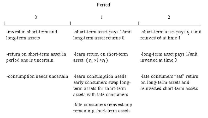
The timeline below illustrates the sequence of investment, returns, and
consumption
2.1
Given the above saving environment, the planner at time zero collects each
saver’s unit and invests s
o
per saver in the short-term asset and 1 s
o
per
saver in the long-term asset. At time one, when the short-term rate r
i
is
realized, the planner can reinvest some fraction s
i
of the short-term asset
until time two. Reinvestment will be state contingent, hence the subscript.
The planner also chooses consumption each period, and consumption will be
state dependent as well. The …rst-period consumption constraint in state i
is
c
1i
= (s
o
s
i
)=:
Early consumers get the short-term investment, less the amount that gets
reinvested until period two. Consumption gets scaled up by because the
planner invests s per saver but only the fraction consume early. Late con-
sumers get the return on the long-term asset and on any short-term assets
6
that were rolled over from the period one, hence the second period consump-
tion constraint is
c
2i
= (1 s
o
+ r
i
s
i
)=(1 ):
The only other constraint on the planner is that reinvestment in both states
must be nonnegative:
s
i
0:
Subject to the three constraints above, the planner chooses fs
0;
s
i
; c
1i
; c
2i
g to
maximize the representative saver’s expected utility at time zero:
EU(c
ti
) = [U(c
1l
) + (1 )U(c
2l
)] + (1 ) [U(c
1h
) + (1 )U(c
2h
)] :
Except for the state-contingent aspect, this is a straightforward programming
problem. The …rst-order conditions can be combined as follows,
s
i
i
= 0; (2)
U
0
(c
1l
) r
l
U
0
(c
2l
) =
l
=; (3)
U
0
(c
1h
) r
h
U
0
(c
2h
) =
h
=(1 ); (4)
(1 ) [U
0
(c
1h
) U
0
(c
2h
)] = [U
0
(c
2l
) U
0
(c
1l
)] ; (5)
where
i
is the multiplier on the constraint that s
i
0: Conditions (3) and
(4) are the combined …rst order conditions for c
ti
and s
i
; while (5) is the
…rst-order condition for s
o
:
The planner’s reinvestment strategy for the short-term asset is contingent
on the rate realized at time one: if that rate turns out low, optimal reinvest-
ment is zero; if it turns out high, reinvestment is positive (see appendix for
proof). Since s
h
> 0,
h
= 0 so (4) implies
U
0
(c
1h
)=U
0
(c
2h
) = r
h
(6)
This standard intertemporal e¢ ciency condition has the planner transfer
goods from period one to p eriod two (by rolling over the short-term asset)
until the marginal (social) rate of substitution between the two types of
consumers equals the marginal rate of transformation. Since r
h
> 1 then
c
1h
< c
2h
implying late consumers get more of the bene…t from the high
return on the short-term asset. On the other hand, s
l
= 0 implies
l
> 0;
hence c
1l
> c
2l
; early consumer are compensated for their sacri…ce in the
7

high return state by higher consumption in the low return state. It turns
out that when savers invest on their own, without the bene…t of a planner
or intermediary, they violate (6); c
1h
is too high and c
2h
is too low b ecause
of inadequate reinvestment when the short-term return turns out high.
5
Substituting (6) into (5) yields
[U
0
(c
2l
) U
0
(c
1l
)] = (1 )[r
h
1]U
0
(c
2h
): (7)
This condition equates the marginal cost and bene…t of investing in the short-
term asset. The left side is the opp ortunity cost of having invested in the
short-term asset on the downside (when the future short-term rate turns out
low); instead of reinvesting the short-term asset, the planner pays out the
return to early consumers, raising their utility by U
0
(c
1l
): Had the planner
invested in the long-term asset instead, he would have paid the unit return
to the late consumers, which raises their utility by U
0
(c
2l
). Because c
2l
< c
1l
,
the opportunity cost of the short-term asset on the downside is positive.
6
The right side of (7) is the net marginal bene…t of the short-term asset when
the return turns out high. When the return is high, the planner reinvests the
short-term asset and earns r
h
. Had he invested more in the long-term asset
at time zero he would have earned only 1, so the extra unit of short-term
asset raises long-term consumers’utility by (r
h
1)U
0
(c
2h
): At the optimal
portfolio, the marginal cost of the short-term asset on the downside (when
the return is low) equals the marginal bene…t on the upside (when the return
is high.)
The optimal portfolio and consumptions are determined as follows. Since
s
l
= 0 and s
h
> 0; consumption in the low return state depends only on s
0
while consumption in the high return state depends on reinvestment as well:
c
1l
= s
o
=;
c
2l
= (1 s
o
)=(1 );
c
1h
= (s
o
s
h
)=;
c
2h
= (1 s
o
+ r
h
s
h
)=(1 ):
5
Since the short-term return on the deposit is random, the contract bears some resem-
blance the the lottery/deposits in Guillen and Tshoegl (2002), although the motivation
for the random element is very di¤erent.
6
The low short-term rate, r
l
; does not enter the equation because the planner never
invests at that rate; he pays out all the short-term asset in that state to early consumers.
8
Substituting those equations into (6) and (7) determines the …rst best short-
term investment and the optimal amount of reinvestment in the high return
state. That portfolio and reinvestment strategy then determine the …rst best
consumptions.
3 Direct Investment and Trading
We now investigate whether savers can replicate the planner’s solution on
their own by choosing an initial portfolio at time zero and then trading
assets at time one after liquidity needs and the next-period return on the
short-term asset are realized. Fortunately, we only need to characterize the
equilibrium to show where the decentralized solution violates the planner’s
allocation.
A few preliminary observations will simplify the analysis. Since savers
are identical ex ante, they will choose the same initial portfolio at time zero.
At time one, early consumers will want to swap their long-term assets for the
short-term assets held by late consumers. The supply of long-term assets is
inelastic, of course, as they are worthless to early consumers. The demand for
the long-term asset, however, will depend on the realized rate on the short-
term asset, as that rate represents the opportunity cost to late consumers of
trading their short-term assets.
Let p
i
denote the price of a unit of long-term asset in terms of the short-
term assets in interest rate state i: Early consumers get the return on their
short-term asset, plus the income from selling their long-term assets to late
consumers:
c
1i
= s
o
+ p
i
(1 s
o
):
If late consumers each purchase l
i
units of long-term assets in period one in
state i; reinvestment in the short-term asset is
s
i
= s
o
p
i
l
i
:
Reinvestment cannot be negative, hence
s
i
0:
This constraint also ensures that each late consumer has enough short-term
assets to cover his purchases of long-term assets.
9
Late consumers in state i consume the return on their initial long-term
assets, the long-term assets they purchase, and any left-over short-term assets
that they rollover:
c
2i
= 1 s
o
+ l
i
+ r
i
s
i
:
Savers choose c
ti
; s
o
; l
i
; s
i
; to maximize their expected utility at time zero,
subject to the constraints above. The …rst order conditions for c
ti
; l
i
; s
i
can
be combined as follows:
s
i
i
= 0 (8)
(1=p
l
r
l
)U
0
(c
2l
) =
l
=(1 ) (9)
(1=p
h
r
h
)U
0
(c
2h
) =
h
=(1 )(1 ) (10)
These conditions pin down the relationship between reinvestment and
the long-term asset price in a given state. If s
i
> 0 )
i
= 0 ) p
i
= 1=r
i
;
positive reinvestment in state i implies the price of the long-term asset equals
its discounted value in that state; the price could not be lower than 1=r
i
or
late consumers would never reinvest at r
i
. Conversely, if p
i
< 1=r
i
)
i
>
0 ) s
i
= 0 ) p
i
l
i
= s
o
; if the price of long-term asset is less than its
discounted value, reinvestment is zero as long-term savers will trade all their
short-term assets for long-term assets. These observations will be useful
momentarily.
The …rst-order condition for s
o
is:
(1 ) [(1 p
h
)U
0
(c
1h
) + (1 )(r
h
1)U
0
(c
2h
)] +
h
=
[(p
l
1)U
0
(c
1l
) + (1 )(1 r
l
)U
0
(c
2l
)]
l
: (11)
The left side is the expected net bene…t across periods of increasing s
o
by
a unit in the event the short-term return is high. Early consumers get the
unit return less the opportunity cost of having one fewer unit of long-term
asset to sell in period one. If p
h
< 1; as it will be, increasing s
o
bene…ts early
consumers. Late consumers also bene…t on net since they can reinvest the
unit at r
h
> 1. The additional bene…t to late consumers is
h
; the value of
having more short-term assets to trade for long-term assets.
On the right is the bene…t of having increased investment in the long-term
asset when the return on the short-term asset is low. Note that if p
h
< 1;
then it must be that p
l
> 1 or savers would not invest in the long-term asset
10

in period zero.
7
Since p
l
> 1 > r
l
; investing more in the long-term asset
at time zero bene…ts both early consumers and late consumers in the low
return state. The only minus,
l
, is that late consumers would have fewer
short-term assets to trade for long-term assets in period one.
In addition to these ex ante equilibrium conditions, the long-term asset
market in period one must also clear in both interest rate states. Since the
fraction of the population will each supply 1 s
o
units of long-term assets
at time one, the aggregate supply of long term assets is (1s
o
): The fraction
1 of the population each purchase l
i
units of the long-term asset in state
i; so aggregate demand for the long term asset is (1 )l
i
: Aggregate supply
equals aggregate demand when
(1 s
o
) = (1 )l
i
: (12)
To determine if the sp ot market equilibrium matches the …rst best (plan-
ner’s) solution, we conjecture an equilibrium like the …rst best and then check
if the resulting consumption allocations are indeed …rst best. The key feature
of the …rst best is that the planner reinvests in the short-term asset when
short-term rates are high. Accordingly, we conjecture s
h
> 0; which implies
p
h
= 1=r
h
< 1: (13)
At that price, consumption in the high return state is
c
1h
= s
o
+ (1 s
o
)=r
h
; (14)
c
2h
= 1 s
o
+ r
h
s
o
(15)
Late consumption turns out to be independent of the amount of reinvestment
when the long-term asset sells for its full discounted value; late consumers
are indi¤erent between reinvesting or buying long-term assets. Relative con-
sumption in the high state is
c
1h
= c
2h
=r
h
: (16)
For most preferences, this ratio will di¤er from the …rst best ratio deter-
mined by (6). Suppose
7
They would expect to buy long-term assets on the cheap in pe riod one, but would …nd
that none were available, in which case the price would be unbounded, which contradicts
p
l
< 1:
11

U(c) =
c
1
1
(17)
where higher 2 [0; 1) indicates increasing risk aversion. Equation (16) then
implies
U
0
(c
1h
) = r
h
U
0
(c
2h
) < r
h
U
0
(c
2h
):
When savers invest directly at time zero, early consumption is higher than in
the …rst best, which implies too little reinvestment. The inequality implies
that the planner could raise welfare at time one by taking a unit from early
consumers, reinvesting at r
h
; and giving the proceeds to late consumers. Ex
post, however, early consumers would not volunteer the unit since they will
not be around to enjoy the higher second period consumption.
The less risk averse are savers, the greater the commitment problem and
ine¢ ciency associated with direct investing and trading. The ratio c
2h
=c
1h
is
independent of when savers invest directly, but the …rst best ratio c
2h
=c
1h
is decreasing in : Less risk averse savers are more ‡exible about shifting
consumption toward period two in order to exploit the high return on the
short-term asset.
We want to show later that savers’investment decisions are also distorted
on the downside, so we need to characterize their allocations in the low
interest state. Since reinvestment in the low state is zero in the …rst best,
we also conjecture s
l
= 0: If late consumers do not reinvest in the low state,
they must trade all their short-term assets for long term assets: s
o
p
l
l
l
:
Using the latter to eliminate l
l
from (12) implies
p
l
=
s
o
(1 )
(1 s
o
)
: (18)
The price of the long-term asset in the low return state is increasing in the
amount of the short-term asset, and in the fraction of late consumers. More
short-term assets means late consumer have more to bid for long-term asset
and fewer assets to bid on. More late consumers means more bidders and
fewer sellers. Since p
l
> 1, (18) implies s
o
> :
The equilibrium price, portfolio, and other variables are determined as
follows. Given s
l
= 0; we know c
1l
= s
o
= and c
2l
= (1 s
o
)=(1 ): Given
s
h
> 0; we know
h
= 0 and p
h
= 1=r
h
: Substituting those values, (14),
(15), and (9) into (11) produces an equation in s
o
and p
l
. That equation and
(18) determine the optimal short-term investment at time zero and the price
12

that will result in period one. Those values then determine the consumption
allocations. Given s
o
; (12) determines l
h
. Those variables and p
h
determine
reinvestment in the high state: s
h
= s
o
p
h
l
h
:
3.1 Risk Aversion and Investment Distortions
We noted in the intro duction that savers’inability to exploit the high return
on the short-term asset leads them to underinvest in the short-term asset.
Their incentives are also distorted on the downside, when the short-term
return is low, because the market price they face at time one di¤ers from
the shadow price the planner faces at time zero. These distortions are more
severe when savers are less risk averse.
Savers underinvest in the short-term asset because the upside bene…t is
too low and the downside cost is too high. Savers’ commitment problem
prevents them from fully exploiting the high return, which lowers the upside
bene…t of the short-term asset. The opportunity cost of the short-term asset
is too high on the downside because the long–term asset sells for more than
one in that state.
We illustrate these distortions under the assumption of constant risk aver-
sion. Even in that case, the extent of nonlinearity in the …rst order conditions
precludes a closed form solution for s
o
: Instead, we reduce the …rst order con-
ditions to a single equation in s
o
and compare the properties of the solution
equations in each case.
Using (6) to eliminate s
h
from (7) produces the solution equation for the
…rst best:
f(s
o
) = (1 )(1 1=r
h
)j(r
h
)g(r
h
s
o
); (19)
Let s
o
denote the solution to (19). The on the left and the (1 ) on
the right indicate that the planner determines s
o
by weighing the downside
against the upside. On the downside, the marginal opportunity cost of the
short-term asset is
f(:)
1
1 s
o
s
o
:
This is the gain in utility from increasing long-term investment and giving
the proceeds to late consumers; f is positive (since s
o
> ) and increasing in
s
o
: The bene…t on the upside depends on
g(:) 1=(1 + (r
h
1)s
o
)
;
13

the gain in utility from increasing short-term investment, reinvesting at r
h
;
and paying the return to late consumers. Note that g is decreasing in s
o
.
The comparable equation for the market solution comes from substituting
the equilibrium long-term asset price (12) into their …rst order (11) (plus the
substitutions described above):
h(s
o
) = (1 )(1 1=r
h
)k(r
h
)g(r
h
s
o
): (20)
The marginal cost of the short term asset on the downside is
h(:)
(1 s
o
)
1
1 s
o
+ s
o
s
o
s
o
s
o
(1 s
o
)
:
Increasing s
o
has two partially o¤setting e¤ects on h: The term in square
brackets is the sum of late consumers’and early consumers’marginal utility,
weighted by the asset shares. Raising s
o
lowers this term since more weight is
placed on early consumers, whose marginal utility declines with s
o
: Increasing
s
o
also increases the price of the long-term asset, however, which increases
the opportunity cost of investing in the short-term asset. The net e¤ect is
positive, so h is increasing in s
o
Comparing the bene…ts and costs reveals why savers underinvest in the
short term asset. The only di¤erence on the upside is between
j(:)
r
h
+ (1 )r
1=
h
and
k(:) r
h
+ (1 )r
h
:
Because x
is concave and < 1; j > k.
8
. The upside is too low because
savers reinvest too little. The di¤erence on the downside for given s
o
is
h(s
o
) f(s
o
) = (p
l
1)(
s
o
)
+1
;
where p
l
is the price of the long term asset in the low interest rate state. The
shadow price to the planner at time zero is one. Since p
l
> 1; the marginal
cost of the short-term asset on the downside is too high. The high cost on the
downside and the low bene…t on the upside both cause savers to underinvest
in the short-term asset.
8
Let x = r
h
and x
0
= r
1=
h
. Then j = (x + (1 )x
0
)
> x
+ (1 )x
0
= k:
14

Note that the distortions on each side are independent. Suppose savers
had access to a better short-term asset with a higher upside return, r
h
, but
the same downside risk, . The bene…t increases with r
h
but the costs do not
change. Suppose the upside on the new asset was high enough to compensate
direct investors for their inability to fully exploit the high return. In this
case, the upside bene…t on the new asset to savers is equivalent to the upside
bene…t on the old asset to the planner.
9
Savers would cho ose s
0
o
of the new
short-term asset, less s
o
, because the cost on the downside is still too high
(relative to the planner).
The cost on the downside is too high because the asset will sell for more
than one, the price to the planner. The high opportunity cost to savers leads
them to underinvest in the asset. Note that if participation were limited,
as in Diamond (1997), the long-term asset price would be lower and the
distortion on the downside would be reduced.
The di¤erence between the optimal portfolio and the savers’own portfolio
is decreasing in the degree of risk aversion. The only case in which the
distortion is zero is when U = ln c. In that case, in which case (6) implies
c
2h
= r
h
c
1h
, the same as under direct investment: We stress this so it will be
understood that …nancial intermediaries here are not providing insurance.
4 Financial Intermediaries
Delegating their investment decisions to an intermediary will almost always
raise savers’expected utility and may give them the …rst best level of welfare.
Savers deposit their wealth at time zero with the intermediary, who o¤ers
savers a two-period contract. The contracting problem facing the interme-
diary is the same as the allocation problem the planner solves except the
intermediary cannot observe a savers’investment horizon at time one.
10
Pri-
vate investment horizons create an incentive problem: if short-term investors
who must withdraw early earn too much, long-term investors will also with-
9
If the upside on the new asset is r
hh
; the bene…t curves are coincident if:
(1 1=r
hh
)k(r
hh
)g(r
hh
s
o
) = (1 1=r
h
)j(r
h
)g(r
h
s
o
):
10
There are no …xed costs to intermediation so there is free entry. Competition among
intermediaries ensures th at the survivors must o¤er contracts that maximize savers’ex-
pected utility at time zero.
15

draw early and reinvest until period two. To prevent this, the contract o¤ered
by the intermediary must satisfy the following incentive constraint:
r
i
c
1i
c
2i
: (21)
Because the intermediary’s problem is a constrained version of the plan-
ner’s, we only need to test if the additional constraint binds in the …rst best in
either state. Savers’preferences will in‡uence whether the constraints binds.
If U(c) = c
1
=(1 ) and < 1; the incentive constraint is slack in the
high return state. With those preferences, (6) implies c
2h
= r
h
c
1h
< r
h
c
1h
so (21) is not binding. Positive reinvestment in the high return state shifts
consumption toward perio d two, which relaxes the incentive constraint.
The incentive constraint may bind in the low state, however. The plan-
ner does not reinvest in that state, so the ratio c
1l
=c
2l
may be high enough
to violate (21). If so, the intermediary must reduce short-term investment
and increase long-term investment.
11
Substituting c
1l
= s
o
= and c
2l
=
(1 s
o
)=(1 ) into (21) determines the intermediary’s maximum incentive
compatible short-term investment:
s
o
=
+ (1 )r
l
:
The upper limit on short-term investment falls as r
l
rises; a higher downside
increases the return to reinvestment so the intermediary must reduce the
amount available for late consumers to reinvest. Higher increases the upper
limit because the short-term investment gets spread across more consumers.
The intermediary achieves the …rst best if s
o
falls to the right of s
o
: If
s
o
> s
o
, the downside cost of the short-term asset exceeds the upside bene…t
so the intermediary would not want to hold s
o
in the …rst place. If s
o
> s
o
;
the intermediary cannot achieve the …rst best but he still dominates direct
investment except when savers happen to choose s
o
on their own.
12
11
Reinvesting in the short-term asset would also relax the incentive constraint, but
investing more in the long-term asset is the most e¢ cient way to raise second period
consumption. Reinvestment is determined by (6) even if the incentive constraint binds.
12
Evaluating (19) at s
o
produces a condition on the parameters that determines whether
the intermediary achieves the …rst best:
s
o
7 s
o
()
(1=r
l
1)
(r
h
+ (1 )r
l
)
? (1 )(1 1=r
h
)j(r
h
):
16

Our intermediaries serve a very di¤erent role from the banks in Dia-
mond and Dybvig (1983). The intermediaries in their model shift the rela-
tively higher return from longer-term assets to early consumers, which allows
smoother consumption. The intermediaries here do just the opposite; they
allow savers to exploit temporary high returns and to shift consumption from
early in life to later in life, which causes more variable consumption.
4.1 Necessary conditions for intermediation
Uncertainty about the timing of consumption needs is necessary before savers
need an intermediary. If there is only uncertainty about returns, but not
about the timing of consumption needs, savers can do just as well by investing
directly. Suppose savers know when they will need to consume in either
period one or two. The solution is trivial; if all savers are early consumers
( = 1); they invest only in the short-term asset. If all savers are late
consumers ( = 0), they will invest only in the long-term asset since it has
the highest expected return. In this case there is obviously no need for an
intermediary.
Intermediaries are necessary only if early consumers get zero utility from
later consumption. Only in that extreme case are savers completely unwill-
ing ex post to substitute late consumption for early consumption. Suppose
instead that savers get utility from consuming in both periods, but we de…ne
early consumers as people with relatively high marginal rates of substitu-
tion between early and late consumption, U
0
(c
1
)=U
0
(c
2
). In that case, savers
could still invest directly in the short-term asset. After they learn rates,
both types would set U
0
(c
1
)=U
0
(c
2
) = r
2
. Consumption allocations would
di¤er, but with the marginal rate of substitution for each type equal to the
marginal rate of transformation ex post, there are no gains to locking up the
short-term asset with an intermediary. Putting it di¤erently, savers would
make the same investments in period one that they would make in period
zero, so there is no commitment problem, and no need for an intermediary.
The contract o¤ered by the intermediary here resembles the callable CDs
now sold by real-world banks.
13
Callable CDs give banks’ a prepayment
option, i.e., they can pay o¤ before the stated maturity date. The option
may exist only for the …rst year of the contract, or until maturity. Bankers’
13
See Certi…cates of Deposits: Tips for Investors,http://www.sec.gov/consumer/certi…c.htm
These callable CDS di¤er from the market indexed CDs analyzed by Chen and Kensigner
(1990).
17

decision whether to call a CD and the CD holders’spending will depend on
market rates much like the contract and consumption allocations modelled
here. If market rates fall (relative to initial CD rate), banks will tend to
call CDs and the holders will tend to spend more (rather than rollover their
savings at the lower rate). If market rates rise, banks will be less inclined to
call CDs, and the holders will postpone consumption. The motivations for
the real-world contract and ours may di¤er, but the e¤ects are similar.
4.2 Another option
As in Boyd and Prescott (1986), the intermediary in our model is essentially
a contract among a coalition of savers. The contract is not unique. Savers
could invest directly in the long term asset and buy an option to sell it the
next period in case they need to consume early. This would solve the essential
purpose of the intermediary: locking up the liquid asset out of reach of early
consumers. This forward market does as well as the intermediary, but the
arrangement is certainly more complicated.
The option market works as follows. In period one, investors divide their
wealth between the short term asset and the long term asset. They can also
buy an option at time zero to sell the long-term asset in period one in state i
for a price of q
i
: Late consumers get a rebate of R
i
: Savers pay a dealer a fee
of f at time zero for this option. The dealer invests the fee in the short-term
asset. Fee revenues must be su¢ cient to buy up all the early consumers
long-term assets. Any excess revenue is reinvested in the short-term asset.
The proceeds from reinvestment are rebated to late consumers, along with
the long-term assets purchased from early consumers.
We can show that the equilibrium contract can deliver the …rst-best by
manipulating the budget constraints of the consumers and dealers.
14
The
"trick" is to show that combined constraints on savers and the dealers re-
duce to the consumption constraints on the planners’problem. This option
14
Since the option dealer cannot observe the savers’type, he faces the same incentive
constraint as the intermediary. This condition ensures that late consumer will not exercise
the option and then reinvest the proceeds in the short-term asset. This constraint will be
just as tight under the option market as under the intermediary. Since the option price will
di¤er from the price that would prevail on the spot market, late consumer might also have
an arbitrage opportunity; they could exercise the option to sell their long-term assets and
then repurchase them from early consumers on the spot market. But the spot market will
never open. If q
i
< p
i
, long-term consumers would not want to buy on the s pot market.
And if q
i
> p
i
; early consumers not want to sell on the spot market.
18
contract gives early consumers
c
1l
= q
i
(1 s
o
) + s
o
:
The dealer must collect enough in fees to purchase the long term assets
from the households that want to sell in period one: f > q
i
l
o
. Let
s
i
denote any excess fees that are reinvested in the short-term asset. The
dealer’s …rst period constraint is
s
i
f q
i
l
o
> 0:
Eliminating q
i
l
o
from these two equations implies
c
1i
= f s
i
+ s
o
:
Consumption by late consumers is
c
2i
= 1 s
o
+ r
i
s
o
+ R
i:
(22)
The dealer must earn enough on reinvestment and the long-term assets they
buy in period one to pay this rebate to the 1 households that consume
late:
(1 )R
i
= r
i
s
i
+ (1 s
o
):
Eliminating R
i
from these two equations implies
(1 )c
2i
= 1 s
o
+ r
i
s
i
+ (1 )r
i
s
o
: (23)
Note that if s
o
= 0, the consumption constraints (22) and (23) are the
same as in the planner’s problem. Let s
denote the …rst best level of in-
vestment in the short-term asset. The solution to the option contract is the
same, as long as f = s
: The crucial feature of the solution is that savers
do not hold the short-term asset directly. This prevents them from consum-
ing the proceeds if they need to consume early. Direct investment in the
long-term asset poses no problems because savers cannot consume that asset
prematurely.
Unlike the intermediary, which invests in both the short-term and long-
term asset in period zero, the option dealer would invest only in the short-
term asset at time zero. The dealer equilibrium is still intermediated in some
sense, however, because savers never invest directly in the short-term asset,
nor do they trade assets among themselves.
19
5 Conclusion
Apart from their roles as diversi…ers, information producers, and liquidity
providers, …nancial intermediaries may serve a more basic "piggy bank" func-
tion for savers. Locking funds in an intermediary, whether a bank CD, a pen-
sion plan, or an insurance annuity, may help some savers stick to long-term
plans that they could not commit to if they held funds directly. Obviously,
these intermediaries attract funds for other reasons, namely the higher re-
turn they may o¤er. Our point is that the illiquidity premium demanded by
some savers may not be as large as one might expect, since for some savers,
illiquidity may be a blessing in disguise.
20
References
[1] Allen, Franklin (1997), "Financial Markets, Intermediaries, and In-
tertemporal Smoothing," Journal of Political Economy, 105 (3), pages
523-46.
[2] Barro, Robert J (1997) "Myopia and Inconsistency in the NewClassical
Growth Model," National Bureau of Economic Research, Working paper
# 6317.
[3] Bernanke, Ben and Mark Gertler (1987) "Banking in General Equilib-
rium" in New Approaches to Monetary Economics, edited by William
A. Barnett and Kenneth J. Singleton. New York, Cambridge University
Press.
[4] Boyd, John H. and Edward C. Prescott (1986) "Financial Intermediary
Coalitions," Journal of Economic Theory, 38, 211-232.
[5] Bryant, J (1980) "A Model of Reserves, Bank Runs, and Deposit Insur-
ance
´
," Journal of Banking and Finance, 4, 335-344.
[6] Chen, Andrew and John W. Kensinger (1990) "An Analyisis of Market-
Indexed Certi…cates of Deposit," Journal of Financial Services Research
[7] Diamond, Douglas, W. (1984) "Financial Intermediation and Delegated
Monitoring," Review of Economic Studies, 51, 393-414.
[8] Diamond, Douglas, W. and Philip Dybvig (1983) "Bank Runs, Deposit
Insurance, and Liquidity." Journal of Political Economy, 91 401-19.
[9] Diamond, Douglas, W. (1997) "Liquidity, Banks, and Markets," Journal
of Political Economy, 105, 928-956.
[10] Guillen, Mario and Adrian Tshoegl (2002) "Banking on Gambling:
Banks and Lottery Linked Accounts," Journal of Financial Services Re-
search, 21:3, 219-231
[11] Hellwig, Martin, "Liquidity Provision, Banking, and The Allocation of
Interest Rate Risk," European Economic Review, (August 1994), 1363-
89.
21
[12] Holmstrom Bengt and Jean Tirole (1998) "Private and Public Supply
of Liquidity," Journal of Political Economy, 1-40.
[13] Laibson, David. (1997) "Golden Eggs and Hyperbolic Discounting,"
Quarterly Journal of Economics, 117, 443-478.
[14] Wallace, Neil (1990), "A Banking Model Where Partial Suspension is
Best," Quarterly Review, Federal Reserve Bank of Minneapolis, 11-23
6 Appendix
This appendix states and proves four lemmas useful in simplifying the plan-
ner’s …rst order conditions for the optimal investment and consumption al-
locations.
Lemma 1 s
l
> 0 ) s
h
> 0: Proof: assume s
l
> 0; s
h
= 0: Then c
1l
> c
2l
and c
1h
< c
2h .
It follows from c
1l
> c
2l
and r
l
< 1 that (1 )= > (1
s
0
+ r
1
s
l
)=(s
0
s
l
) > (1 s
0
)=s
0
but c
1h
< c
2h
) (1 )= > (1 s
0
)=s
0
;a
contradiction.
Lemma 2 s
l
) c
1l
> c
21
by (2) and (3) while s
h
= 0 ) c
1h
< c
2h
by (2) and
(4): c
1l
> c
21
and r
l
< 1 ) (1 )= > (1 s
0
+ r
1
s
l
)=(s
0
s
l
) > (1 s
0
)=s
0
while c
1h
< c
2h
) (1 )= < (1 s
0
)=s
0
; a contradiction.
Lemma 3 s
l
> 0 ) c
2l
< c
2h
: Proof: assume s
l
> 0; c
2
_
l
> c
2h
:
Since c
2l
< c
1l
and c
2h
> c
1h
(by lemma 1), c
2h
< c
2l
) c
1l
> c
1h
:
But c
2
_
l
> c
2h
) r
h
s
h
< r
l
s
l
) s
l
> s
h
) c
1l
< c
1h
; a contradiction.
Lemma 4 s
l
= 0: Proof: s
l
> 0 ) s
h
> 0 (by Lemma 1), hence
l
=
l
= 0:
Conditions (3), (4), and (5) ) (1 )(r
h
1)=(1 r
l
) = U
0
(c
2l
)=U
0
(c
2h
) >
1(by Lemma 2),
which is a contradiction, as r
h
< 1:
Lemma 5 s
h
> 0: Proof: Suppose s
h
= s
l
= 0 ) c
1l
= c
1h
c
1
and c
2l
=
c
1h
c
2
: Condition (5) ) U
0
(c
1
) = U
0
(c
2
), while (5) ) U
0
(c
1
) > U
0
(c
2
), a
contradiction.
22
