
637
Chapter 11
Electrochemical Methods
Chapter Overview
11A Overview of Electrochemistry
11B Potentiometric Methods
11C Coulometric Methods
11D Voltammetric and Amperometric Methods
11E Key Terms
11F Chapter Summary
11G Problems
11H Solutions to Practice Exercises
In Chapter 10 we examined several spectroscopic techniques that take advantage of the
interaction between electromagnetic radiation and matter. In this chapter we turn our attention
to electrochemical techniques in which the potential, current, or charge in an electrochemical
cell serves as the analytical signal.
Although there are only three fundamental electrochemical signals, there are many possible
experimental designs—too many, in fact, to cover adequately in an introductory textbook.
e simplest division of electrochemical techniques is between bulk techniques, in which we
measure a property of the solution in the electrochemical cell, and interfacial techniques, in
which the potential, current, or charge depends on the species present at the interface between
an electrode and the solution in which it sits. e measurement of a solution’s conductivity,
which is proportional to the total concentration of dissolved ions, is one example of a bulk
electrochemical technique. A determination of pH using a pH electrode is an example of an
interfacial electrochemical technique. Only interfacial electrochemical methods receive further
consideration in this chapter.

638
Analytical Chemistry 2.1
11A Overview of Electrochemistry
e focus of this chapter is on analytical techniques that use a measurement
of potential, current, or charge to determine an analyte’s concentration or
to characterize an analyte’s chemical reactivity. Collectively we call this area
of analytical chemistry because its originated from the
study of the movement of electrons in an oxidation–reduction reaction.
Despite the dierence in instrumentation, all electrochemical tech-
niques share several common features. Before we consider individual ex-
amples in greater detail, let’s take a moment to consider some of these
similarities. As you work through the chapter, this overview will help you
focus on similarities between dierent electrochemical methods of analysis.
You will nd it easier to understand a new analytical method when you can
see its relationship to other similar methods.
11A.2 Five Important Concepts
To understand electrochemistry we need to appreciate ve important and
interrelated concepts: (1) the electrode’s potential determines the analyte’s
form at the electrode’s surface; (2) the concentration of analyte at the elec-
trode’s surface may not be the same as its concentration in bulk solution;
(3) in addition to an oxidation–reduction reaction, the analyte may partici-
pate in other chemical reactions; (4) current is a measure of the rate of the
analyte’s oxidation or reduction; and (5) we cannot control simultaneously
current and potential.
The elecTrode’s PoTenTial deTermines The analyTe’s Form
In Chapter 6 we introduced the ladder diagram as a tool for predicting
how a change in solution conditions aects the position of an equilibrium
reaction. Figure 11.1, for example, shows a ladder diagram for the Fe
3+
/
Fe
2+
and the Sn
4+
/Sn
2+
equilibria. If we place an electrode in a solution
of Fe
3+
and Sn
4+
and adjust its potential to +0.500 V, Fe
3+
is reduced to
Fe
2+
but Sn
4+
is not reduced to Sn
2+
.
e material in this section—particularly
the ve important concepts—draws upon
a vision for understanding electrochem-
istry outlined by Larry Faulkner in the
article “Understanding Electrochemistry:
Some Distinctive Concepts,” J. Chem.
Educ. 1983, 60, 262–264.
See also, Kissinger, P. T.; Bott, A. W.
“Electrochemistry for the Non-Electro-
chemist,” Current Separations, 2002, 20:2,
51–53.
You may wish to review the earlier treat-
ment of oxidation–reduction reactions
in Section 6D.4 and the development of
ladder diagrams for oxidation–reduction
reactions in Section 6F.3.
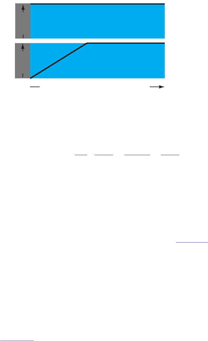
Figure 11.1 Redox ladder diagram for Fe
3+
/Fe
2+
and for Sn
4+
/
Sn
2+
redox couples. e areas in blue show the potential range
where the oxidized forms are the predominate species; the re-
duced forms are the predominate species in the areas shown in
pink. Note that a more positive potential favors the oxidized
forms. At a potential of +0.500 V (green arrow) Fe
3+
reduces
to Fe
2+
, but Sn
4+
remains unchanged.
E
E
o
Sn
4+
/Sn
2+
= +0.154 V
E
o
Fe
3+
/Fe
2+
= +0.771V
Fe
3+
Fe
2+
Sn
4+
Sn
2+
more negative
more positive
+0.500 V
639
Chapter 11 Electrochemical Methods
inTerFacial concenTraTions may noT equal Bulk concenTraTions
In Chapter 6 we introduced the Nernst equation, which provides a math-
ematical relationship between the electrode’s potential and the concentra-
tions of an analyte’s oxidized and reduced forms in solution. For example,
the Nernst equation for Fe
3+
and Fe
2+
is
[]
[]
.
[]
[]
ln logEE
nF
RT
1
0 05916
Fe
Fe
Fe
Fe
Fe /Fe
o
3
2
3
2
32
=- =
+
+
+
+
++
11.1
where E is the electrode’s potential and
E
Fe /Fe
o
32++
is the standard-state re-
duction potential for the reaction
() () eaq aqFe Fe
32
? +
++-
. Because it is
the potential of the electrode that determines the analyte’s form at the
electrode’s surface, the concentration terms in equation 11.1 are those of
Fe
2+
and Fe
3+
at the electrode's surface, not their concentrations in bulk
solution.
is distinction between a species’ surface concentration and its bulk
concentration is important. Suppose we place an electrode in a solution of
Fe
3+
and x its potential at 1.00 V. From the ladder diagram in Figure 11.1,
we know that Fe
3+
is stable at this potential and, as shown in Figure 11.2a,
the concentration of Fe
3+
is the same at all distances from the electrode’s
surface. If we change the electrode’s potential to +0.500 V, the concentra-
tion of Fe
3+
at the electrode’s surface decreases to approximately zero. As
shown in Figure 11.2b, the concentration of Fe
3+
increases as we move
away from the electrode’s surface until it equals the concentration of Fe
3+
in bulk solution. e resulting concentration gradient causes additional
Fe
3+
from the bulk solution to diuse to the electrode’s surface.
The analyTe may ParTiciPaTe in oTher reacTions
Figure 11.1 and Figure 11.2 shows how the electrode’s potential aects
the concentration of Fe
3+
and how the concentration of Fe
3+
varies as a
function of distance from the electrode’s surface. e reduction of Fe
3+
to
Fe
2+
, which is governed by equation 11.1, may not be the only reaction
that aects the concentration of Fe
3+
in bulk solution or at the electrode’s
surface. e adsorption of Fe
3+
at the electrode’s surface or the formation
Figure 11.2 Concentration of Fe
3+
as a function of dis-
tance from the electrode’s surface at (a) E = +1.00 V and
(b) E = +0.500 V. e electrode is shown in gray and
the solution in blue.
We call the region of solution that contains
this concentration gradient in Fe
3+
the dif-
fusion layer. We will have more to say about
this in Section 11D.2.
bulk
solution
diusion
layer
(a)
(b)
distance from electrode’s surface
[Fe
3+
]
[Fe
3+
]
bulk
solution

640
Analytical Chemistry 2.1
of a metal–ligand complex in bulk solution, such as Fe(OH)
2+
, also aects
the concentration of Fe
3+
.
currenT is a measure oF raTe
e reduction of Fe
3+
to Fe
2+
consumes an electron, which is drawn from
the electrode. e oxidation of another species, perhaps the solvent, at a
second electrode is the source of this electron. Because the reduction of
Fe
3+
to Fe
2+
consumes one electron, the ow of electrons between the elec-
trodes—in other words, the current—is a measure of the rate at which Fe
3+
is reduced. One important consequence of this observation is that the cur-
rent is zero when the reaction
() ()
e
aq aq
Fe Fe
32
? +
++-
is at equilibrium.
We cannoT conTrol simulTaneously BoTh The currenT and The PoTenTial
If a solution of Fe
3+
and Fe
2+
is at equilibrium, the current is zero and the
potential is given by equation 11.1. If we change the potential away from
its equilibrium position, current ows as the system moves toward its new
equilibrium position. Although the initial current is quite large, it decreases
over time, reaching zero when the reaction reaches equilibrium. e cur-
rent, therefore, changes in response to the applied potential. Alternatively,
we can pass a xed current through the electrochemical cell, forcing the
reduction of Fe
3+
to Fe
2+
. Because the concentrations of Fe
3+
decreases
and the concentration of Fe
2+
increases, the potential, as given by equation
11.1, also changes over time. In short, if we choose to control the potential,
then we must accept the resulting current, and we must accept the resulting
potential if we choose to control the current.
11A.2 Controlling and Measuring Current and Potential
Electrochemical measurements are made in an electrochemical cell that
consists of two or more electrodes and the electronic circuitry needed to
control and measure the current and the potential. In this section we intro-
duce the basic components of electrochemical instrumentation.
e simplest electrochemical cell uses two electrodes. e potential of
one electrode is sensitive to the analyte’s concentration, and is called the
or the . e second electrode,
which we call the , completes the electrical circuit and
provides a reference potential against which we measure the working elec-
trode’s potential. Ideally the counter electrode’s potential remains constant
so that we can assign to the working electrode any change in the overall
cell potential. If the counter electrode’s potential is not constant, then we
replace it with two electrodes: a whose potential
remains constant and an that completes the electri-
cal circuit.
Because we cannot control simultaneously the current and the poten-
tial, there are only three basic experimental designs: (1) we can measure
e rate of the reaction
() ()aq aq eFe Fe
32
? +
++-
is the change in the concentration of Fe
3+
as a function of time.

641
Chapter 11 Electrochemical Methods
the potential when the current is zero, (2) we can measure the potential
while we control the current, and (3) we can measure the current while we
control the potential. Each of these experimental designs relies on O’
, which states that the current, i, passing through an electrical circuit of
resistance, R, generates a potential, E.
EiR=
Each of these experimental designs uses a dierent type of instrument.
To help us understand how we can control and measure current and po-
tential, we will describe these instruments as if the analyst is operating them
manually. To do so the analyst observes a change in the current or the
potential and manually adjusts the instrument’s settings to maintain the
desired experimental conditions. It is important to understand that modern
electrochemical instruments provide an automated, electronic means for
controlling and measuring current and potential, and that they do so by
using very dierent electronic circuitry than that described here.
PoTenTiomeTers
To measure the potential of an electrochemical cell under a condition of
zero current we use a . Figure 11.3 shows a schematic
diagram for a manual potentiometer that consists of a power supply, an
electrochemical cell with a working electrode and a counter electrode, an
ammeter to measure the current that passes through the electrochemical
cell, an adjustable, slide-wire resistor, and a tap key for closing the circuit
through the electrochemical cell. Using Ohm’s law, the current in the upper
half of the circuit is
i
R
E
ab
upper
PS
=
is point bears repeating: It is impor-
tant to understand that the experimental
designs in Figure 11.3, Figure 11.4, and
Figure 11.5 do not represent the elec-
trochemical instruments you will nd in
today’s analytical labs. For further infor-
mation about modern electrochemical
instrumentation, see this chapter’s addi-
tional resources.
Figure 11.3 Schematic diagram of a manual potentiometer: C is
the counter electrode; W is the working electrode; SW is a slide-
wire resistor; T is a tap key and i is an ammeter for measuring
current.
i
a bc
Electrochemical
Cell
C
W
T
SW
Power
Supply

642
Analytical Chemistry 2.1
where E
PS
is the power supply’s potential, and R
ab
is the resistance between
points a and b of the slide-wire resistor. In a similar manner, the current in
the lower half of the circuit is
i
R
E
cb
lower
cell
=
where E
cell
is the potential dierence between the working electrode and
the counter electrode, and R
cb
is the resistance between the points c and b
of the slide-wire resistor. When i
upper
= i
lower
= 0, no current ows through
the ammeter and the potential of the electrochemical cell is
E
R
R
E
ab
cb
cell PS
#=
11.2
To determine E
cell
we briey press the tap key and observe the current at
the ammeter. If the current is not zero, then we adjust the slide wire resistor
and remeasure the current, continuing this process until the current is zero.
When the current is zero, we use equation 11.2 to calculate E
cell
.
Using the tap key to briey close the circuit through the electrochemical
cell minimizes the current that passes through the cell and limits the change
in the electrochemical cell’s composition. For example, passing a current of
10
–9
A through the electrochemical cell for 1 s changes the concentrations
of species in the cell by approximately 10
–14
moles. Modern potentiometers
use operational ampliers to create a high-impedance voltmeter that mea-
sures the potential while drawing a current of less than 10
–9
A.
GalvanosTaTs
A , a schematic diagram of which is shown in Figure 11.4, al-
lows us to control the current that ows through an electrochemical cell.
e current from the power supply through the working electrode is
i
RR
E
cell
PS
=
+
where E
PS
is the potential of the power supply, R is the resistance of the
resistor, and R
cell
is the resistance of the electrochemical cell. If R >> R
cell
,
then the current between the auxiliary and working electrodes
i
R
E
constant
PS
.=
maintains a constant value. To monitor the working electrode’s potential,
which changes as the composition of the electrochemical cell changes, we
can include an optional reference electrode and a high-impedance poten-
tiometer.
PoTenTiosTaTs
A , a schematic diagram of which is shown in Figure 11.5
allows us to control the working electrode’s potential. e potential of the
working electrode is measured relative to a constant-potential reference
electrode that is connected to the working electrode through a high-im-
Figure 11.4 Schematic diagram
of a galvanostat: A is the auxiliary
electrode; W is the working elec-
trode; R is an optional reference
electrode, E is a high-impedance
potentiometer, and i is an amme-
ter. e working electrode and the
optional reference electrode are
connected to a ground.
Electrochemical
Cell
A
W
Power
Supply
R
i
E
resistor

643
Chapter 11 Electrochemical Methods
pedance potentiometer. To set the working electrode’s potential we adjust
the slide wire resistor that is connected to the auxiliary electrode. If the
working electrode’s potential begins to drift, we adjust the slide wire resistor
to return the potential to its initial value. e current owing between the
auxiliary electrode and the working electrode is measured with an ammeter.
Modern potentiostats include waveform generators that allow us to apply
a time-dependent potential prole, such as a series of potential pulses, to
the working electrode.
11A.3 Interfacial Electrochemical Techniques
Because interfacial electrochemistry is such a broad eld, let’s use Figure
11.6 to organize techniques by the experimental conditions we choose to
use (Do we control the potential or the current? How do we change the
applied potential or applied current? Do we stir the solution?) and the
analytical signal we decide to measure (Current? Potential?).
At the rst level, we divide interfacial electrochemical techniques into
static techniques and dynamic techniques. In a static technique we do not
allow current to pass through the electrochemical cell and, as a result, the
concentrations of all species remain constant. Potentiometry, in which we
measure the potential of an electrochemical cell under static conditions, is
one of the most important quantitative electrochemical methods and is
discussed in detail in section 11B.
Dynamic techniques, in which we allow current to ow and force a
change in the concentration of species in the electrochemical cell, comprise
the largest group of interfacial electrochemical techniques. Coulometry, in
which we measure current as a function of time, is covered in Section 11C.
Amperometry and voltammetry, in which we measure current as a function
of a xed or variable potential, is the subject of Section 11D.
Figure 11.5 Schematic diagram for a manual potentiostat: W is the
working electrode; A is the auxiliary electrode; R is the reference elec-
trode; SW is a slide-wire resistor, E is a high-impendance potentiom-
eter; and i is an ammeter.
i
Electrochemical
Cell
A
W
SW
Power
Supply
R
E

644
Analytical Chemistry 2.1
11B Potentiometric Methods
In potentiometry we measure the potential of an electrochemical cell under
static conditions. Because no current—or only a negligible current—ows
through the electrochemical cell, its composition remains unchanged. For
this reason, potentiometry is a useful quantitative method of analysis. e
rst quantitative potentiometric applications appeared soon after the for-
mulation, in 1889, of the Nernst equation, which relates an electrochemical
cell’s potential to the concentration of electroactive species in the cell.
1
Potentiometry initially was restricted to redox equilibria at metallic
electrodes, which limited its application to a few ions. In 1906, Cremer
discovered that the potential dierence across a thin glass membrane is a
function of pH when opposite sides of the membrane are in contact with
solutions that have dierent concentrations of H
3
O
+
. is discovery led to
the development of the glass pH electrode in 1909. Other types of mem-
branes also yield useful potentials. For example, in 1937 Koltho and Sand-
ers showed that a pellet of AgCl can be used to determine the concentration
of Ag
+
. Electrodes based on membrane potentials are called ion-selective
electrodes, and their continued development extends potentiometry to a
diverse array of analytes.
1 Stork, J. T. Anal. Chem. 1993, 65, 344A–351A.
interfacial
electrochemical techniques
static techniques
(i = 0)
dynamic techniques
(i ≠ 0)
potentiometry
controlled
potential
controlled
current
variable
potential
xed
potential
stirred
solution
quiescent
solution
hydrodynamic
voltammetry
stripping
voltammetry
polarography and
stationary electrode
voltammetry
pulse polarography
and voltammetry
cyclic
voltammetry
controlled-current
coulometry
amperometry
controlled-potential
coulometry
measure E
measure i vs. E
measure i vs. t
measure i
measure i vs. E
measure i vs. E
measure i vs. E
measure i vs. E
measure i vs. t
linear potential pulsed potential
cyclical potential
Figure 11.6 Family tree that highlights the similarities
and dierences between a number of interfacial electro-
chemical techniques. e specic techniques are shown
in red, the experimental conditions are shown in blue,
and the analytical signals are shown in green.
For an on-line introduction to much of the
material in this section, see Analytical Elec-
trochemistry: Potentiometry by Erin Gross,
Richard S. Kelly, and Donald M. Cannon,
Jr., a resource that is part of the Analytical
Sciences Digital Library.
645
Chapter 11 Electrochemical Methods
11B.1 Potentiometric Measurements
As shown in Figure 11.3, we use a potentiometer to determine the dier-
ence between the potential of two electrodes. e potential of one elec-
trode—the working or indicator electrode—responds to the analyte’s ac-
tivity and the other electrode—the counter or reference electrode—has a
known, xed potential. In this section we introduce the conventions for
describing potentiometric electrochemical cells, and the relationship be-
tween the measured potential and the analyte’s activity.
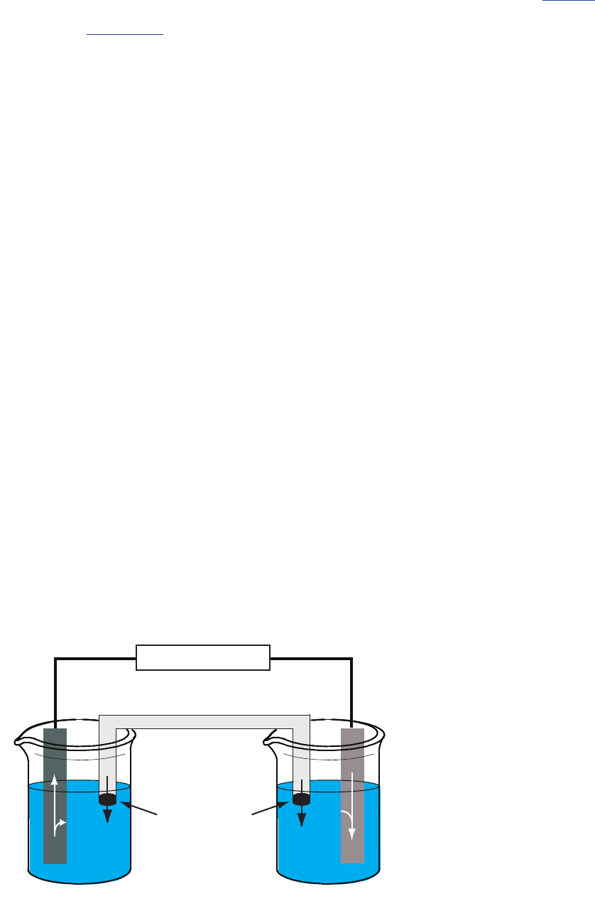
PoTenTiomeTric elecTrochemical cells
A schematic diagram of a typical potentiometric electrochemical cell is
shown in Figure 11.7. e electrochemical cell consists of two half-cells,
each of which contains an electrode immersed in a solution of ions whose
activities determine the electrode’s potential. A that contains
an inert electrolyte, such as KCl, connects the two half-cells. e ends of
the salt bridge are xed with porous frits, which allow the electrolyte’s ions
to move freely between the half-cells and the salt bridge. is movement of
ions in the salt bridge completes the electrical circuit.
By convention, we identify the electrode on the left as the and
assign to it the oxidation reaction; thus
() ()
esa
q
Zn Zn 2
2
? +
+-
e electrode on the right is the , where the reduction reaction
occurs.
() ()eaq sAg Ag?+
+-
e potential of the electrochemical cell in Figure 11.7 is for the reaction
() () ()
()
saqs aq
Zn 2Ag2Ag Zn
2
?++
++
We also dene potentiometric electrochemical cells such that the cathode is
the indicator electrode and the anode is the reference electrode.
Figure 11.7 Example of a potentiometric electro-
chemical cell. e activities of Zn
2+
and Ag
+
are
shown below the two half-cells.
e reason for separating the electrodes
is to prevent the oxidation reaction and
the reduction reaction from occurring at
one of the electrodes. For example, if we
place a strip of Zn metal in a solution of
AgNO
3
, the reduction of Ag
+
to Ag oc-
curs on the surface of the Zn at the same
time as a potion of the Zn metal oxidizes
to Zn
2+
. Because the transfer of electrons
from Zn to Ag
+
occurs at the electrode’s
surface, we can not pass them through the
potentiometer.
In Chapter 6 we noted that a chemical
reaction’s equilibrium position is a func-
tion of the activities of the reactants and
products, not their concentrations. To be
correct, we should write the Nernst equa-
tion in terms of activities. So why didn’t
we use activities in Chapter 9 when we
calculated redox titration curves? ere
are two reasons for that choice. First, con-
centrations are always easier to calculate
than activities. Second, in a redox titration
we determine the analyte’s concentration
from the titration’s end point, not from
the potential at the end point. e only
reasons for calculating a titration curve
is to evaluate its feasibility and to help us
select a useful indicator. In most cases, the
error we introduce by assuming that con-
centration and activity are identical is too
small to be a signicant concern.
In potentiometry we cannot ignore the
dierence between activity and concen-
tration. Later in this section we will con-
sider how we can design a potentiometric
method so that we can ignore the dier-
ence between activity and concentration.
See Chapter 6I to review our earlier dis-
cussion of activity and concentration.
potentiometer
salt bridge
porous frits
KCl
Cl
-
K
+
Zn
Zn
2+
2e
-
Ag
Ag
+
e
-
a
Zn
2+ = 0.0167 a
Ag
+ = 0.100
Cl
-
Cl
-
anode cathode
NO
3
–

646
Analytical Chemistry 2.1
shorThand noTaTion For elecTrochemical cells
Although Figure 11.7 provides a useful picture of an electrochemical cell,
it is not a convenient way to represent it. A more useful way to describe an
electrochemical cell is a shorthand notation that uses symbols to identify
dierent phases and that lists the composition of each phase. We use a
vertical slash (|) to identify a boundary between two phases where a po-
tential develops, and a comma (,) to separate species in the same phase or
to identify a boundary between two phases where no potential develops.
Shorthand cell notations begin with the anode and continue to the cathode.
For example, we describe the electrochemical cell in Figure 11.7 using the
following shorthand notation.
() ()aasaqaqsZn ZnCl (, 0.0167) AgNO (, 0.100) Ag
2Zn3Ag
2
;<;==
++
e double vertical slash (||) represents the salt bridge, the contents of which
we usually do not list. Note that a double vertical slash implies that there is
a potential dierence between the salt bridge and each half-cell.
Example 11.1
What are the anodic, the cathodic, and the overall reactions responsible
for the potential of the electrochemical cell in Figure 11.8? Write the
shorthand notation for the electrochemical cell.
Solution
e oxidation of Ag to Ag
+
occurs at the anode, which is the left half-cell.
Because the solution contains a source of Cl
–
, the anodic reaction is
() ()
e
aq s
Ag Cl AgCl?++
+- -
e cathodic reaction, which is the right half-cell, is the reduction of Fe
3+
to Fe
2+
.
Imagine having to draw a picture of each
electrochemical cell you are using!
Figure 11.8 Potentiometric electrochemical
cell for Example 11.1.
potentiometer
salt bridge
KCl
Pt
Ag
HCl
AgCl(s)
FeCl
2
FeCl
3
a
Cl
– = 0.100
a
Fe
2+ = 0.0100
a
Fe
3+ = 0.0500

647
Chapter 11 Electrochemical Methods
() ()eaq aqFe Fe
32
?+
+-+
e overall cell reaction, therefore, is
() () () () ()
saqaqsaq
Ag Fe Cl AgCl Fe
32
?++ +
+- +
e electrochemical cell’s shorthand notation is
(, .),()
(, .),(,.)
()
()
a
aq aaqa
saq
s
0 100
0 0100 0 0500
Ag HClAgCl
FeCl FeCl Pt
sat'd
Cl
2Fe3Fe
23
;<
;
=
==
-
++
Note that the Pt cathode is an inert electrode that carries electrons to the
reduction half-reaction. e electrode itself does not undergo reduction.
Practice Exercise 11.1
Write the reactions occurring at the anode and the cathode for the poten-
tiometric electrochemical cell with the following shorthand notation.
,
() () () ()
()
sgaq aq s
Pt HH Cu Cu
2
2
;<;
++
Click here to review your answer to this exercise.
PoTenTial and acTiviTy—The nernsT equaTion
e potential of a potentiometric electrochemical cell is
EE E
cell cathodeanode
=-
11.3
where E
cathode
and E
anode
are reduction potentials for the redox reactions
at the cathode and the anode, respectively. Each reduction potential are is
by the Nernst equation
lnEE
nF
RT
Q
o
=-
where E
o
is the standard-state reduction potential, R is the gas constant,
T is the temperature in Kelvins, n is the number of electrons in the redox
reaction, F is Faraday’s constant, and Q is the reaction quotient. At a tem-
perature of 298 K (25
o
C) the Nernst equation is
.
logEE
n
Q
0 05916
o
=-
11.4
where E is in volts.
Using equation 11.4, the potential of the anode and cathode in Figure
11.7 are
.
logEE
a2
0 05916
1
anode
Zn /Zn
o
Zn
2
2
=-
+
+
.
logEE
a1
0 05916
1
cathode
Ag /Ag
o
Ag
=-
+
+
Substituting E
cathode
and E
anode
into equation 11.3, along with the activities
of Zn
2+
and Ag
+
and the standard-state reduction potentials, gives E
cell
as
..
lo
gl
ogEE
a
E
a1
0 05916
1
2
0 05916
1
cell
Ag /Ag
o
Ag
Zn /Zn
o
Zn
2
2
=- --
+
+
+
+
aa
kk
See Section 6D.4 for a review of the
Nernst equation.
Even though an oxidation reaction is
taking place at the anode, we dene the
anode's potential in terms of the cor-
responding reduction reaction and the
standard-state reduction potential. See
Section 6D.4 for a review of using the
Nernst equation in calculations.
You will nd values for the standard-state
reduction potential in Appendix 13.

648
Analytical Chemistry 2.1
.
.
.
.
.
.
.
log
log
E 0 7996
1
0 05916
0 100
1
0 7618
2
0 05916
0 0167
1
1 555
V
VV
cell
=- -
-- =+
a
a
k
k
Example 11.2
What is the potential of the electrochemical cell shown in Example 11.1?
Solution
Substituting E
cathode
and E
anode
into equation 11.3, along with the concen-
trations of Fe
3+
, Fe
2+
, and Cl
–
and the standard-state reduction potentials
gives
..
lo
gl
ogEE
a
a
Ea
1
0 05916
1
0 05916
cell
Fe /Fe
o
Fe
Fe
AgCl/Ag
o
Cl
3
2
32
=- --
++
+
+
-
a
a
k
k
.
.
.
.
.
.
(.
).
log
log
E 0 771
1
0 05916
0 0500
0 0100
0 2223
1
0 05916
0 100 0 531
V
VV
cell
=- -
-=
+
a
a
k
k
Practice Exercise 11.2
What is the potential for the electrochemical cell in Practice Exercise 11.1
if the activity of H
+
in the anodic half-cell is 0.100, the fugacity of H
2
in the anodic half-cell is 0.500, and the activity of Cu
2+
in the cathodic
half-cell is 0.0500?
Click here to review your answer to this exercise.
Fugacity is the equivalent term for the ac-
tivity of a gas.
In potentiometry, we assign the reference electrode to the anodic half-
cell and assign the indicator electrode to the cathodic half-cell. us, if the
potential of the cell in Figure 11.7 is +1.50 V and the activity of Zn
2+
is
0.0167, then we can solve the following equation for a
Ag
+
..
.
.
.
.
log
log
a
15007996
1
0 05916
1
0 7618
2
0 05916
0 0167
1
VV
Ag
=- -
--
+
a
a
k
k
obtaining an activity of 0.0118.
Example 11.3
What is the activity of Fe
3+
in an electrochemical cell similar to that in
Example 11.1 if the activity of Cl
–
in the left-hand cell is 1.0, the activity
of Fe
2+
in the right-hand cell is 0.015, and E
cell
is +0.546 V?
Solution
Making appropriate substitutions into equation 11.3

649
Chapter 11 Electrochemical Methods
..
..
.
.
(.)
log
log
a
0 546 0 771
1
0 05916 0010
0 2223
1
0 05916
10
5
VV
V
Fe
3
=- -
-
+
a
a
k
k
and solving for a
Fe
3+ gives its activity as 0.0135.
Practice Exercise 11.3
What is the activity of Cu
2+
in the electrochemical cell in Practice Exer-
cise 11.1 if the activity of H
+
in the anodic half-cell is 1.00 with a fugacity
of 1.00 for H
2
, and an E
cell
of +0.257 V?
Click here to review your answer to this exercise.
Despite the apparent ease of determining an analyte’s activity using
the Nernst equation, there are several problems with this approach. One
problem is that standard-state potentials are temperature-dependent and
the values in reference tables usually are for a temperature of 25
o
C. We can
overcome this problem by maintaining the electrochemical cell at 25
o
C or
by measuring the standard-state potential at the desired temperature.
Another problem is that a standard-sate reduction potential may have a
signicant matrix eect. For example, the standard-state reduction poten-
tial for the Fe
3+
/Fe
2+
redox couple is +0.735 V in 1 M HClO
4
, +0.70 V
in 1 M HCl, and +0.53 V in 10 M HCl. e dierence in potential for
equimolar solutions of HCl and HClO
4
is the result of a dierence in
the activity coecients for Fe
3+
and Fe
2+
in these two media. e shift
toward a more negative potential with an increase in the concentration of
HCl is the result of chloride’s ability to form a stronger complex with Fe
3+
than with Fe
2+
. We can minimize this problem by replacing the standard-
state potential with a matrix-dependent formal potential. Most tables of
standard-state potentials, including those in Appendix 13, include selected
formal potentials.
Finally, a more serious problem is the presence of additional potentials
in the electrochemical cell not included in equation 11.3. In writing the
shorthand notation for an electrochemical cell we use a double slash (||) to
indicate the salt bridge, suggesting a potential exists at the interface between
each end of the salt bridge and the solution in which it is immersed. e
origin of this potential is discussed in the following section.
JuncTion PoTenTials
A develops at the interface between two ionic solution
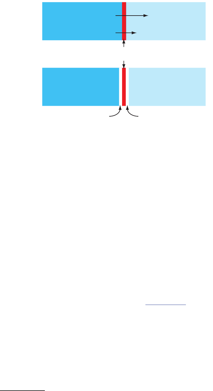
if there dierence in the concentration and mobility of the ions. Consider,
for example, a porous membrane that separations a solution of 0.1 M HCl
from a solution of 0.01 M HCl (Figure 11.9a). Because the concentration
of HCl on the membrane’s left side is greater than that on the right side of
the membrane, H
+
and Cl
–
will diuse in the direction of the arrows. e
e standard-state reduction potentials in
Appendix 13, for example, are for 25
o
C.
650
Analytical Chemistry 2.1
mobility of H
+
, however, is greater than that for Cl
–
, as shown by the dif-
ference in the lengths of their respective arrows. Because of this dierence in
mobility, the solution on the right side of the membrane develops an excess
concentration of H
+
and a positive charge (Figure 11.9b). Simultaneously,
the solution on the membrane’s left side develops a negative charge because
there is an excess concentration of Cl
–
. We call this dierence in potential
across the membrane a junction potential and represent it as E
j
.
e magnitude of the junction potential depends upon the dierence
in the concentration of ions on the two sides of the interface, and may be
as large as 30–40 mV. For example, a junction potential of 33.09 mV has
been measured at the interface between solutions of 0.1 M HCl and 0.1 M
NaCl.
2
A salt bridge’s junction potential is minimized by using a salt, such
as KCl, for which the mobilities of the cation and anion are approximately
equal. We also can minimize the junction potential by incorporating a
high concentration of the salt in the salt bridge. For this reason salt bridges
frequently are constructed using solutions that are saturated with KCl. Nev-
ertheless, a small junction potential, generally of unknown magnitude, is
always present.
When we measure the potential of an electrochemical cell, the junction
potential also contributes to E
cell
; thus, we rewrite equation 11.3 as
EE EE
jcell cathodeanode
=-+
to include its contribution. If we do not know the junction potential’s
actual value—which is the usual situation—then we cannot directly cal-
culate the analyte’s concentration using the Nernst equation. Quantitative
analytical work is possible, however, if we use one of the standardization
methods discussed in Chapter 5C.
2 Sawyer, D. T.; Roberts, J. L., Jr. Experimental Electrochemistry for Chemists, Wiley-Interscience:
New York, 1974, p. 22.
Figure 11.9 Origin of the junction potential be-
tween a solution of 0.1 M HCl and a solution of
0.01 M HCl.
0.1 M HCl 0.01 M HCl
porous
membrane
H
+
Cl
–
0.1 M HCl 0.01 M HCl
+
+
+
+
+
+
+
-
-
-
-
-
-
-
excess H
+
excess Cl
–
(a)
(b)
ese standardization methods are ex-
ternal standards, the method of standard
additions, and internal standards. We will
return to this point later in this section.
651
Chapter 11 Electrochemical Methods
11B.2 Reference Electrodes
In a potentiometric electrochemical cell one of the two half-cells provides
a xed reference potential and the potential of the other half-cell responds
the analyte’s concentration. By convention, the reference electrode is the
anode; thus, the short hand notation for a potentiometric electrochemical
cell is
referenceelectrode indicatorelectrode<
and the cell potential is
EEEE
jcell indref
=-+
e ideal reference electrode provides a stable, known potential so that
we can attribute any change in E
cell
to the analyte’s eect on the indicator
electrode’s potential. In addition, it should be easy to make and to use the
reference electrode. ree common reference electrodes are discussed in
this section.
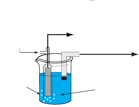
sTandard hydroGen elecTrode
Although we rarely use the (SHE) for
routine analytical work, it is the reference electrode used to establish stan-
dard-state potentials for other half-reactions. e SHE consists of a Pt elec-
trode immersed in a solution in which the activity of hydrogen ion is 1.00
and in which the fugacity of H
2
(g) is 1.00 (Figure 11.10). A conventional
salt bridge connects the SHE to the indicator half-cell. e short hand
notation for the standard hydrogen electrode is
(, .) (, .)
()
gf Haqa
s
100100Pt ,H
2H H
2
;<==
+
+
and the standard-state potential for the reaction
()
()
eaq gH
2
1
H
2
?+
+-
is, by denition, 0.00 V at all temperatures. Despite its importance as
the fundamental reference electrode against which we measure all other
Figure 11.10 Schematic diagram showing the
standard hydrogen electrode.
Pt
KCl
H
2
(g)
fugacity = 1.00
to potentiometer
salt bridge to
indicator half-cell
H
2
(g)
H
+
(activity = 1.00)

652
Analytical Chemistry 2.1
potentials, the SHE is rarely used because it is dicult to prepare and in-
convenient to use.
calomel elecTrodes
A calomel reference electrode is based on the following redox couple be-
tween Hg
2
Cl
2
and Hg
() () ()eslaq2Hg Cl 2Hg2Cl
22
?++
--
for which the potential is
.
() .
.
()
lo
gl
ogEE
aa
2
0 05916
0 2682
2
0 05916
V
Cl Cl
22
Hg Cl /Hg
o
22
=- =+ -
- -
e potential of a calomel electrode, therefore, depends on the activity of
Cl
–
in equilibrium with Hg and Hg
2
Cl
2
.
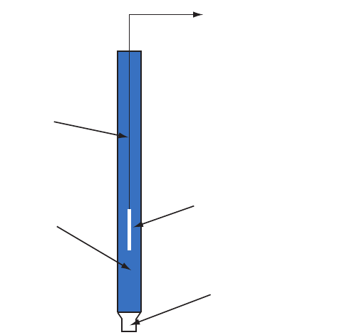
As shown in Figure 11.11, in a (SCE)
the concentration of Cl
–
is determined by the solubility of KCl. e elec-
trode consists of an inner tube packed with a paste of Hg, Hg
2
Cl
2
, and KCl,
situated within a second tube that contains a saturated solution of KCl. A
small hole connects the two tubes and a porous wick serves as a salt bridge
to the solution in which the SCE is immersed. A stopper in the outer tube
provides an opening for adding addition saturated KCl. e short hand
notation for this cell is
,(,)
() ()
aq
ls
Hg Hg Cl KCl sat'd
22
;<
Because the concentration of Cl
–
is xed by the solubility of KCl, the
potential of an SCE remains constant even if we lose some of the inner solu-
tion to evaporation. A signicant disadvantage of the SCE is that the solu-
bility of KCl is sensitive to a change in temperature. At higher temperatures
the solubility of KCl increases and the electrode’s potential decreases. For
example, the potential of the SCE is +0.2444 V at 25
o
C and +0.2376 V
Calomel is the common name for the
compound Hg
2
Cl
2
.
Figure 11.11 Schematic diagram showing the saturated calo-
mel electrode.
to potentiometer
Hg
(l)
saturated KCl(aq)
ll hole
Hg
(l), Hg
2
Cl
2
(s)
, KCl(s)
KCl crystals
hole
porous wick
653
Chapter 11 Electrochemical Methods
at 35
o
C. e potential of a calomel electrode that contains an unsaturated
solution of KCl is less dependent on the temperature, but its potential
changes if the concentration, and thus the activity of Cl
–
, increases due to
evaporation.
silver/silver chloride elecTrodes
Another common reference electrode is the / -
, which is based on the reduction of AgCl to Ag.
() () ()essaqAgCl Ag Cl?++
--
As is the case for the calomel electrode, the activity of Cl
–
determines the
potential of the Ag/AgCl electrode; thus
...loglogEE aa0 05916 0 2223 0 05916V
AgCl/Ag
o
Cl Cl
=- =+ -
- -
When prepared using a saturated solution of KCl, the electrode’s potential
is +0.197 V at 25
o
C. Another common Ag/AgCl electrode uses a solution
of 3.5 M KCl and has a potential of +0.205 V at 25
o
C.
A typical Ag/AgCl electrode is shown in Figure 11.12 and consists of a
silver wire, the end of which is coated with a thin lm of AgCl, immersed
in a solution that contains the desired concentration of KCl. A porous plug
serves as the salt bridge. e electrode’s short hand notation is
(, )() () aq axssAg AgCl ,KCl
Cl
;<=
-
converTinG PoTenTials BeTWeen reFerence elecTrodes
e standard state reduction potentials in most tables are reported relative
to the standard hydrogen electrode’s potential of +0.00 V. Because we
rarely use the SHE as a reference electrode, we need to convert an indicator
For example, the potential of a calomel
electrode is +0.280 V when the concentra-
tion of KCl is 1.00 M and +0.336 V when
the concentration of KCl is 0.100 M. If
the activity of Cl
–
is 1.00, the potential
is +0.2682 V.
Figure 11.12 Schematic diagram showing a Ag/AgCl elec-
trode. Because the electrode does not contain solid KCl, this
is an example of an unsaturated Ag/AgCl electrode.
to potentiometer
Ag wire coated
with AgCl
KCl solution
porous plug
Ag wire
As you might expect, the potential of a
Ag/AgCl electrode using a saturated solu-
tion of KCl is more sensitive to a change
in temperature than an electrode that uses
an unsaturated solution of KCl.

654
Analytical Chemistry 2.1
electrode’s potential to its equivalent value when using a dierent reference
electrode. As shown in the following example, this is easy to do.
Example 11.4
e potential for an Fe
3+
/Fe
2+
half-cell is +0.750 V relative to the stan-
dard hydrogen electrode. What is its potential if we use a saturated calomel
electrode or a saturated silver/silver chloride electrode?
Solution
When we use a standard hydrogen electrode the potential of the electro-
chemical cell is
.. .EE E 0 750 0 000 0 750VV V
cell
o
SHE
Fe /Fe
32
=-=-=+
++
We can use the same equation to calculate the potential if we use a satu-
rated calomel electrode
.. .EE E 0 750 0 2444 0 506VV V
cell
o
SCE
Fe /Fe
32
=-=- =+
++
or a saturated silver/silver chloride electrode
.. .EE E 0 750 0 197 0 553VV V
cell
o
AgCl/Ag
Fe /Fe
32
=- =-=+
++
Figure 11.13 provides a pictorial representation of the relationship be-
tween these dierent potentials.
Figure 11.13 Relationship between the potential of an Fe
3+
/Fe
2+
half-cell relative to the
reference electrodes in Example 11.4. e potential relative to a standard hydrogen elec-
trode is shown in blue, the potential relative to a saturated silver/silver chloride electrode is
shown in red, and the potential relative to a saturated calomel electrode is shown in green.
Practice Exercise 11.4
e potential of a
UO
2
+
/U
4+
half-cell is –0.0190 V relative to a saturated
calomel electrode. What is its potential when using a saturated silver/
silver chloride electrode or a standard hydrogen electrode?
Click here to review your answer to this exercise.
+0.000 V
SHE
+0.197 V
Ag/AgCl
+0.2444 V
SCE
+0.750 V
+0.506 V
+0.553 V
Potential (V)
+0.750 V
Fe
3+
/Fe
2+
// //

655
Chapter 11 Electrochemical Methods
11B.3 Metallic Indicator Electrodes
In potentiometry, the potential of the indicator electrode is proportional to
the analyte’s activity. Two classes of indicator electrodes are used to make
potentiometric measurements: metallic electrodes, which are the subject
of this section, and ion-selective electrodes, which are covered in the next
section.
elecTrodes oF The FirsT kind
If we place a copper electrode in a solution that contains Cu
2+
, the elec-
trode’s potential due to the reaction
()
()e
aq s
2Cu Cu
2
?+
+-
is determined by the activity of Cu
2+
.
.
.
.
lo
gl
ogEE
aa2
0 05916
1
0 3419
2
0 05916
1
V
Cu /Cu
o
Cu Cu
2 2
2
=- =+ -
+
+ +
If copper is the indicator electrode in a potentiometric electrochemical cell
that also includes a saturated calomel reference electrode
(, ) ()aq axsSCECuCu
2
Cu
2
<;=
+
+
then we can use the cell potential to determine an unknown activity of
Cu
2+
in the indicator electrode’s half-cell
.
.
.log
EEEE
a
E0 3419
2
0 05916
1
0 2224
VV
j
j
cell indSCE
Cu
2
=- +=
+-
-+
+
An indicator electrode in which the metal is in contact with a solution
containing its ion is called an . In general, if
a metal, M, is in a solution of M
n+
, the cell potential is
..
lo
gl
ogEK
na
K
n
a
0 05916
1
0 05916
M
Mcell
n
n
=- =+
+
+
where K is a constant that includes the standard-state potential for the
M
n+
/M redox couple, the potential of the reference electrode, and the
junction potential. For a variety of reasons—including the slow kinetics
of electron transfer at the metal–solution interface, the formation of metal
oxides on the electrode’s surface, and interfering reactions—electrodes of
the rst kind are limited to the following metals: Ag, Bi, Cd, Cu, Hg, Pb,
Sn, Tl, and Zn.
elecTrodes oF The second kind
e potential of an electrode of the rst kind responds to the activity of
M
n+
. We also can use this electrode to determine the activity of another
species if it is in equilibrium with M
n+
. For example, the potential of a Ag
electrode in a solution of Ag
+
is
..logEa0 7996 0 05916V
Ag
=+ +
+
11.5
Many of these electrodes, such as Zn,
cannot be used in acidic solutions because
they are easily oxidized by H
+
.
() ()
() ()
saq
gaq
Zn 2H
HZn
2
2
?+
+
+
+
Note that including E
j
in the constant K
means we do not need to know the junc-
tion potential’s actual value; however, the
junction potential must remain constant
if K is to maintain a constant value.

656
Analytical Chemistry 2.1
If we saturate the indicator electrode’s half-cell with AgI, the solubility
reaction
() () ()saqaqAgI Ag I? +
+-
determines the concentration of Ag
+
; thus
a
a
K
Ag
I
sp, AgI
=
+
-
11.6
where K
sp, AgI
is the solubility product for AgI. Substituting equation 11.6
into equation 11.5
..logE
a
K
0 7996 0 05916V
I
sp, AgI
=+ +
-
shows that the potential of the silver electrode is a function of the activity
of I
–
. If we incorporate this electrode into a potentiometric electrochemical
cell with a saturated calomel electrode
(, )
()
()aq axssSCEAgI ,I Ag
I
<;=
-
-
then the cell potential is
.logEK a0 05916
cell I
=-
-
where K is a constant that includes the standard-state potential for the
Ag
+
/Ag redox couple, the solubility product for AgI, the reference elec-
trode’s potential, and the junction potential.
If an electrode of the rst kind responds to the activity of an ion in
equilibrium with M
n+
, we call it an . Two
common electrodes of the second kind are the calomel and the silver/silver
chloride reference electrodes.
redox elecTrodes
An electrode of the rst kind or second kind develops a potential as the
result of a redox reaction that involves the metallic electrode. An electrode
also can serve as a source of electrons or as a sink for electrons in an unre-
lated redox reaction, in which case we call it a . e Pt
cathode in Figure 11.8 and Example 11.1 is a redox electrode because its
potential is determined by the activity of Fe
2+
and Fe
3+
in the indicator
half-cell. Note that a redox electrode’s potential often responds to the activi-
ty of more than one ion, which limits its usefulness for direct potentiometry.
11B.4 Membrane Electrodes
If metals were the only useful materials for constructing indicator elec-
trodes, then there would be few useful applications of potentiometry. In
1906, Cremer discovered that the potential dierence across a thin glass
membrane is a function of pH when opposite sides of the membrane are
in contact with solutions that have dierent concentrations of H
3
O
+
. e
existence of this led to the development of a whole
In an electrode of the second kind we link
together a redox reaction and another re-
action, such as a solubility reaction. You
might wonder if we can link together
more than two reactions. e short answer
is yes. An electrode of the third kind, for
example, links together a redox reaction
and two other reactions. Such electrodes
are less common and we will not consider
them in this text.

657
Chapter 11 Electrochemical Methods
new class of indicator electrodes, which we call -
(ISEs). In addition to the glass pH electrode, ion-selective electrodes are
available for a wide range of ions. It also is possible to construct a mem-
brane electrode for a neutral analyte by using a chemical reaction to gener-
ate an ion that is monitored with an ion-selective electrode. e develop-
ment of new membrane electrodes continues to be an active area of research.
memBrane PoTenTials
Figure 11.14 shows a typical potentiometric electrochemical cell equipped
with an ion-selective electrode. e short hand notation for this cell is
[] (, )[]( ,)()aq ax aq ayref(sample)A Aref internal
samp Aint A
<;<==
where the ion-selective membrane is represented by the vertical slash that
separates the two solutions that contain analyte: the sample solution and
the ion-selective electrode’s internal solution. e potential of this electro-
chemical cell includes the potential of each reference electrode, a junction
potential, and the membrane’s potential
EE EEE
jcell ref(int) ref(samp)mem
=- ++
11.7
where E
mem
is the potential across the membrane. Because the junction
potential and the potential of the two reference electrodes are constant, any
change in E
cell
reects a change in the membrane’s potential.
e analyte’s interaction with the membrane generates a membrane
potential if there is a dierence in its activity on the membrane’s two sides.
Current is carried through the membrane by the movement of either the
analyte or an ion already present in the membrane’s matrix. e membrane
potential is given by the following Nernst-like equation
Figure 11.14 Schematic diagram that shows a typical poten-
tiometric cell with an ion-selective electrode. e ion-selec-
tive electrode’s membrane separates the sample, which con-
tains the analyte at an activity of (a
A
)
samp
, from an internal
solution that contains the analyte with an activity of (a
A
)
int
.
potentiometer
sample
solution
internal
solution
(a)
samp
(a)
int
reference
(sample)
reference
(internal)
ion-selective
membrane
ion-selective
electrode
e notations ref(sample) and ref(internal)
represent a reference electrode immersed
in the sample and a reference electrode
immersed in the ISE’s internal solution.
For now we simply note that a dierence
in the analyte’s activity results in a mem-
brane potential. As we consider dierent
types of ion-selective electrodes, we will
explore more specically the source of the
membrane potential.

658
Analytical Chemistry 2.1
()
()
lnEE
zF
RT
a
a
A
A
memasym
samp
int
=-
11.8
where (a
A
)
samp
is the analyte’s activity in the sample, (a
A
)
int
is the analyte’s
activity in the ion-selective electrode’s internal solution, and z is the ana-
lyte’s charge. Ideally, E
mem
is zero when (a
A
)
int
= (a
A
)
samp
. e term E
asym
,
which is an , accounts for the fact that E
mem
usually
is not zero under these conditions.
Substituting equation 11.8 into equation 11.7, assuming a temperature
of 25
o
C, and rearranging gives
.
()logEK
z
a
0 05916
Acell samp
=+
11.9
where K is a constant that includes the potentials of the two reference elec-
trodes, the junction potentials, the asymmetry potential, and the analyte's
activity in the internal solution. Equation 11.9 is a general equation and
applies to all types of ion-selective electrodes.
selecTiviTy oF memBranes
A membrane potential results from a chemical interaction between the
analyte and active sites on the membrane’s surface. Because the signal de-
pends on a chemical process, most membranes are not selective toward
a single analyte. Instead, the membrane potential is proportional to the
concentration of each ion that interacts with the membrane’s active sites.
We can rewrite equation 11.9 to include the contribution to the potential
of an interferent, I
.
()logEK
z
aKa
0 05916
,
/
A
AAII
zz
cell
AI
=+ +
"
,
where z
A
and z
I
are the charges of the analyte and the interferent, and K
A,I
is a that accounts for the relative response of the
interferent. e selectivity coecient is dened as
()
()
K
a
a
,
/
AI
I
zz
A
e
e
AI
=
11.10
where (a
A
)
e
and (a
I
)
e
are the activities of analyte and the interferent that
yield identical cell potentials. When the selectivity coecient is 1.00, the
membrane responds equally to the analyte and the interferent. A mem-
brane shows good selectivity for the analyte when K
A,I
is signicantly less
than 1.00.
Selectivity coecients for most commercially available ion-selective
electrodes are provided by the manufacturer. If the selectivity coecient is
not known, it is easy to determine its value experimentally by preparing a
series of solutions, each of which contains the same activity of interferent,
(a
I
)
add
, but a dierent activity of analyte. As shown in Figure 11.15, a plot
of cell potential versus the log of the analyte’s activity has two distinct linear
regions. When the analyte’s activity is signicantly larger than K
A,I
�(a
I
)
add
,
See Chapter 3D.4 for an additional dis-
cussion of selectivity.
E
asym
in equation 11.8 is similar to E
o
in
equation 11.1.

659
Chapter 11 Electrochemical Methods
the potential is a linear function of log(a
A
), as given by equation 11.9. If
K
A,I
�(a
I
)
add
is signicantly larger than the analyte’s activity, however, the
cell’s potential remains constant. e activity of analyte and interferent at
the intersection of these two linear regions is used to calculate K
A,I
.
Example 11.5
Sokalski and co-workers described a method for preparing ion-selective
electrodes with signicantly improved selectivities.
3
For example, a con-
ventional Pb
2+
ISE has a logK
Pb
2+
/Mg
2+ of –3.6. If the potential for a
solution in which the activity of Pb
2+
is 4.1�10
–12
is identical to that
for a solution in which the activity of Mg
2+
is 0.01025, what is the value
of logK
Pb
2+
/Mg
2+?
Solution
Making appropriate substitutions into equation 11.10, we nd that
()
()
(. )
.
.K
a
a
0 01025
41 10
40 10
//
zz 22
12
10
Pb /Mg
Mg
e
Pb e
2
2
22
Pb Mg
22
#
#== =
++
-
-
++
+
+
++
e value of logK
Pb
2+
/Mg
2+, therefore, is –9.40.
3 Sokalski, T.; Ceresa, A.; Zwicki, T.; Pretsch, E. J. Am. Chem. Soc. 1997, 119, 11347–11348.
Figure 11.15 Diagram showing the experimental de-
termination of an ion-selective electrode’s selectivity for
an analyte. e activity of analyte that corresponds to
the intersection of the two linear portions of the curve,
(a
A
)
inter
, produces a cell potential identical to that of
the interferent. e equation for the selectivity coef-
cient, K
A,I
, is shown in red.
E
cell
(a
A
)>>K
A,I
×(a
I
)
add
log(a
A
)
(a
A
)<<K
A,I
×(a
I
)
add
K
A,I
=
(a
A
)
e
(a
A
)
inter
z
A
/z
I
(a
I
)
add
(a
I
)
e
z
A
/z
I
=
(a
A
)
inter
Practice Exercise 11.5
A ion-selective electrode for
NO
2
-
has logK
A,I
values of –3.1 for F
–
, –4.1
for
SO
4
2-
, –1.2 for I
–
, and –3.3 for
NO
3
-
. Which ion is the most seri-
ous interferent and for what activity of this interferent is the potential
equivalent to a solution in which the activity of
NO
2
-
is 2.75�10
–4
?
Click here to review your answer to this exercise.

660
Analytical Chemistry 2.1
Glass ion-selecTive elecTrodes
e rst commercial were manufactured using Corning
015, a glass with a composition that is approximately 22% Na
2
O, 6% CaO,
and 72% SiO
2
. When immersed in an aqueous solution for several hours,
the outer approximately 10 nm of the membrane’s surface becomes hy-
drated, resulting in the formation of negatively charged sites, —SiO
–
. So-
dium ions, Na
+
, serve as counter ions. Because H
+
binds more strongly
to —SiO
–
than does Na
+
, they displace the sodium ions
H–SiONa–SiOH Na?++
+-+-++
explaining the membrane’s selectivity for H
+
. e transport of charge
across the membrane is carried by the Na
+
ions. e potential of a glass
electrode using Corning 015 obeys the equation
.logEK a0 05916
cell H
=+
+
11.11
over a pH range of approximately 0.5 to 9. At more basic pH levels the
glass membrane is more responsive to other cations, such as Na
+
and K
+
.
Example 11.6
For a Corning 015 glass membrane, the selectivity coecient K
H
+
/Na
+ is
≈ 10
–11
. What is the expected error if we measure the pH of a solution in
which the activity of H
+
is 2 � 10
–13
and the activity of Na
+
is 0.05?
Solution
A solution in which the actual activity of H
+
, (a
H
+)
act
, is 2 � 10
–13
has a
pH of 12.7. Because the electrode responds to both H
+
and Na
+
, the ap-
parent activity of H
+
, (a
H
+)
app
, is
() () ()
(.)
aaKa
21010005 710
act
13 11 13
Happ HH/NaNa
#
###
=+ =
+=
-- -
++++ +
e apparent activity of H
+
is equivalent to a pH of 12.2, an error of –0.5
pH units.
Replacing Na
2
O and CaO with Li
2
O and BaO extends the useful pH range
of glass membrane electrodes to pH levels greater than 12.
Glass membrane pH electrodes often are available in a combination
form that includes both the indicator electrode and the reference electrode.
e use of a single electrode greatly simplies the measurement of pH. An
example of a typical combination electrode is shown in Figure 11.16.
e observation that the Corning 015 glass membrane responds to
ions other than H
+
(see Example 11.6) led to the development of glass
membranes with a greater selectivity for other cations. For example, a glass
membrane with a composition of 11% Na
2
O, 18% Al
2
O
3
, and 71% SiO
2
is used as an ion-selective electrode for Na
+
. Other glass ion-selective elec-
pH = –log(a
H
+)

661
Chapter 11 Electrochemical Methods
trodes have been developed for the analysis of Li
+
, K
+
, Rb
+
, Cs
+
,
NH
4
+
,
Ag
+
, and Tl
+
. Table 11.1 provides several examples.
Because an ion-selective electrode’s glass membrane is very thin—it is
only about 50 µm thick—they must be handled with care to avoid cracks
or breakage. Glass electrodes usually are stored in a storage buer recom-
mended by the manufacturer, which ensures that the membrane’s outer
surface remains hydrated. If a glass electrode dries out, it is reconditioned
by soaking for several hours in a solution that contains the analyte. e
composition of a glass membrane will change over time, which aects the
electrode’s performance. e average lifetime for a typical glass electrode
is several years.
Figure 11.16 Schematic diagram showing a combination glass
electrode for measuring pH. e indicator electrode consists
of a pH-sensitive glass membrane and an internal Ag/AgCl
reference electrode in a solution of 0.1 M HCl. e sample’s
reference electrode is a Ag/AgCl electrode in a solution of KCl
(which may be saturated with KCl or contain a xed concen-
tration of KCl). A porous wick serves as a salt bridge between
the sample and its reference electrode.
to meter
0.1 M HCl
porous wick
Ag/AgCl reference
electrode (internal)
Ag/AgCl reference
electrode (sample)
KCl solution
pH-sensitive
glass membrane
Table 11.1 Representative Examples of Glass Membrane Ion-
Selective Electrodes for Analytes Other than H
+
analyte membrane composition selectivity coecients
a
Na
+
11% Na
2
O, 18% Al
2
O
3
, 71% SiO
2
K
Na
+
/H
+ = 1000
K
Na
+
/K
+ = 0.001
K
Na
+
/Li
+ = 0.001
Li
+
15% Li
2
O, 25% Al
2
O
3
, 60% SiO
2
K
Li
+
/Na
+ = 0.3
K
Li
+
/K
+ = 0.001
K
+
27% Na
2
O, 5% Al
2
O
3
, 68% SiO
2
K
K
+
/Na
+
= 0.05
a
Selectivity coecients are approximate; values found experimentally may vary substantially from the
listed values. See Cammann, K. Working With Ion-Selective Electrodes, Springer-Verlag: Berlin, 1977.

662
Analytical Chemistry 2.1
solid-sTaTe ion-selecTive elecTrodes
A - - has a membrane that consists
of either a polycrystalline inorganic salt or a single crystal of an inorganic
salt. We can fashion a polycrystalline solid-state ion-selective electrode by
sealing a 1–2 mm thick pellet of Ag
2
S—or a mixture of Ag
2
S and a second
silver salt or another metal sulde—into the end of a nonconducting plas-
tic cylinder, lling the cylinder with an internal solution that contains the
analyte, and placing a reference electrode into the internal solution. Figure
11.17 shows a typical design.
e membrane potential for a Ag
2
S pellet develops as the result of a
dierence in the extent of the solubility reaction
() ()
()
sa
qa
q
Ag S2Ag S
2
2
? +
+-
on the membrane’s two sides, with charge carried across the membrane by
Ag
+
ions. When we use the electrode to monitor the activity of Ag
+
, the
cell potential is
.logEK a0 05916
cell Ag
=+
+
e membrane also responds to the activity of S
2–
, with a cell potential of
.
logEK a
2
0 05916
cell S
2
=-
-
If we combine an insoluble silver salt, such as AgCl, with the Ag
2
S, then
the membrane potential also responds to the concentration of Cl
–
, with a
cell potential of
.logEK a0 05916
cell Cl
=-
-
By mixing Ag
2
S with CdS, CuS, or PbS, we can make an ion-selective
electrode that responds to the activity of Cd
2+
, Cu
2+
, or Pb
2+
. In this case
the cell potential is
.
lnEK a
2
0 05916
Mcell
2
=+
+
where a
M
2+ is the activity of the metal ion.
Table 11.2 provides examples of polycrystalline, Ag
2
S-based solid-state
ion-selective electrodes. e selectivity of these ion-selective electrodes
depends on the relative solubility of the compounds. A Cl
–
ISE using a
Ag
2
S/AgCl membrane is more selective for Br
–
(K
Cl
–
/Br
– = 10
2
) and for
I
–
(K
Cl
–
/I
– = 10
6
) because AgBr and AgI are less soluble than AgCl. If the
activity of Br
–
is suciently high, AgCl at the membrane/solution interface
is replaced by AgBr and the electrode’s response to Cl
–
decreases substan-
tially. Most of the polycrystalline ion-selective electrodes listed in Table
11.2 operate over an extended range of pH levels. e equilibrium between
S
2–
and HS
–
limits the analysis for S
2–
to a pH range of 13–14.
e membrane of a F
–
ion-selective electrode is fashioned from a single
crystal of LaF
3
, which usually is doped with a small amount of EuF
2
to
e NaCl in a salt shaker is an example of
polycrystalline material because it consists
of many small crystals of sodium chlo-
ride. e NaCl salt plates shown in Figure
10.32a, on the other hand, are an example
of a single crystal of sodium chloride.
Figure 11.17 Schematic diagram of a solid-
state electrode. e internal solution con-
tains a solution of analyte of xed activity.
to meter
Ag/AgCl
reference electrode
internal
solution of analyte
membrane
plastic cylinder

663
Chapter 11 Electrochemical Methods
enhance the membrane’s conductivity. Because EuF
2
provides only two
F
–
ions—compared to the three F
–
ions in LaF
3
—each EuF
2
produces a
vacancy in the crystal’s lattice. Fluoride ions pass through the membrane by
moving into adjacent vacancies. As shown in Figure 11.17, the LaF
3
mem-
brane is sealed into the end of a non-conducting plastic cylinder, which
Table 11.2 Representative Examples of Polycrystalline Solid-
State Ion-Selective Electrodes
analyte membrane composition selectivity coecients
a
Ag
+
Ag
2
S
K
Ag
+
/Cu
2+ = 10
–6
K
Ag
+
/Pb
2+ = 10
–10
Hg
2
+
interferes
Cd
2+
CdS/Ag
2
S
K
Cd
2+
/Fe
2+ = 200
K
Cd
2+
/Pb
2+ = 6
Ag
+
, Hg
2
+
, and Cu
2+
must be absent
Cu
2+
CuS/Ag
2
S
K
Cu
2+
/Fe
3+ = 10
K
Cd
2+
/Cu
+ = 1
Ag
+
and Hg
2
+
must be absent
Pb
2+
PbS/Ag
2
S
K
Pb
2+
/Fe
3+ = 1
K
Pb
2+
/Cd
2+ = 1
Ag
+
, Hg
2
+
, and Cu
2+
must be absent
Br
–
AgBr/Ag
2
S
K
Br
–
/I
– = 5000
K
Br
–
/Cl
– = 0.005
K
Br
–
/OH
– = 10
–5
S
2–
must be absent
Cl
–
AgCl/Ag
2
S
K
Cl
–
/I
– = 10
6
K
Cl
–
/Br
– = 100
K
Cl
–
/OH
– = 0.01
S
2–
must be absent
I
–
AgI/Ag
2
S
K
I
–
/S
2– = 30
K
I
–
/Br
– = 10
–4
K
I
–
/Cl
– = 10
–6
K
I
–
/OH
– = 10
–7
SCN
–
AgSCN/Ag
2
S
K
SCN
–
/I
– = 10
3
K
SCN
–
/Br
– = 100
K
SCN
–
/Cl
– = 0.1
K
SCN
–
/OH
– = 0.01
S
2–
must be absent
S
2–
Ag
2
S Hg
2
+
interferes
a
Selectivity coecients are approximate; values found experimentally may vary substantially from the
listed values. See Cammann, K. Working With Ion-Selective Electrodes, Springer-Verlag: Berlin, 1977.

664
Analytical Chemistry 2.1
contains a standard solution of F
–
, typically 0.1 M NaF, and a Ag/AgCl
reference electrode.
e membrane potential for a F
–
ISE results from a dierence in the
solubility of LaF
3
on opposite sides of the membrane, with the potential
given by
.logEK a0 05916
cell F
=-
-
One advantage of the F
–
ion-selective electrode is its freedom from in-
terference. e only signicant exception is OH
–
(K
F
–
/OH
– = 0.1), which
imposes a maximum pH limit for a successful analysis.
Example 11.7
What is the maximum pH that we can tolerate if we need to analyze a solu-
tion in which the activity of F
–
is 1�10
–5
with an error of less than 1%?
Solution
In the presence of OH
–
the cell potential is
.EK aK a0 05916
cell FF/O
HO
H
#=- +
--
--
"
,
To achieve an error of less than 1%, the term K
F
–
/OH
– �a
OH
– must be less
than 1% of a
F
–; thus
.Ka a001
F/OH OH F
###
--
--
..(. )a010001 10 10
5
OH
###
#
-
-
Solving for a
OH
– gives the maximum allowable activity for OH
–
as 1�10
–6
,
which corresponds to a pH of less than 8.
Practice Exercise 11.6
Suppose you wish to use the nitrite-selective electrode in Practice Ex-
ercise 11.5 to measure the activity of
NO
2
-
. If the activity of
NO
2
-
is
2.2 � 10
–4
, what is the maximum pH you can tolerate if the error due
to OH
–
must be less than 10%? e selectivity coecient for OH
–
,
K
NO /OH
2
-
-
, is 630. Do you expect the electrode to have a lower pH limit?
Clearly explain your answer.
Click here to review your answer to this exercise.
Below a pH of 4 the predominate form of uoride in solution is HF, which
does not contribute to the membrane potential. For this reason, an analysis
for uoride is carried out at a pH greater than 4.
Unlike a glass membrane ion-selective electrode, a solid-state ISE does
not need to be conditioned before it is used, and it may be stored dry. e
surface of the electrode is subject to poisoning, as described above for a
Cl
–
ISE in contact with an excessive concentration of Br
–
. If an electrode
is poisoned, it can be returned to its original condition by sanding and
polishing the crystalline membrane.
Poisoning simply means that the surface
has been chemically modied, such as
AgBr forming on the surface of a AgCl
membrane.

665
Chapter 11 Electrochemical Methods
liquid-Based ion-selecTive elecTrodes
Another class of ion-selective electrodes uses a hydrophobic membrane that
contains a liquid organic complexing agent that reacts selectively with the
analyte. ree types of organic complexing agents have been used: cat-
ion exchangers, anion exchangers, and neutral ionophores. A membrane
potential exists if the analyte’s activity is dierent on the two sides of the
membrane. Current is carried through the membrane by the analyte.
One example of a - - is that for
Ca
2+
, which uses a porous plastic membrane saturated with the cation ex-
changer di-(n-decyl) phosphate. As shown in Figure 11.18, the membrane
is placed at the end of a non-conducting cylindrical tube and is in contact
with two reservoirs. e outer reservoir contains di-(n-decyl) phosphate
in di-n-octylphenylphosphonate, which soaks into the porous membrane.
e inner reservoir contains a standard aqueous solution of Ca
2+
and a
Ag/AgCl reference electrode. Calcium ion-selective electrodes also are avail-
able in which the di-(n-decyl) phosphate is immobilized in a polyvinyl
chloride (PVC) membrane that eliminates the need for the outer reservoir.
e membrane potential for the Ca
2+
ISE develops as the result of a
dierence in the extent of the complexation reaction
() ()
()
aq me
mm
em
Ca 2(CHO) PO Ca[(C HO)PO]
2
10 21 2
2
10 21 2
2
?+
+- -
on the two sides of the membrane, where (mem) indicates a species that
is present in the membrane. e cell potential for the Ca
2+
ion-selective
electrode is
.
logEK a
2
0 05916
cell Ca
2
=+
+
e selectivity of this electrode for Ca
2+
is very good, with only Zn
2+
show-
ing greater selectivity.
Figure 11.18 Schematic diagram showing a liq-
uid-based ion-selective electrode for Ca
2+
. e
structure of the cation exchanger, di-(n-decyl)
phosphate, is shown in red.
to meter
Ag/AgCl
reference electrode
membrane saturated with
di-(n-decyl) phosphate
reservoir containing
di-(n-decyl) phosphate
P
O
O
O O
standard
solution of Ca
2+
An is a ligand whose exterior
is hydrophobic and whose interior is hy-
drophilic. e crown ether shown here
O
O
O
O
O
is one example of an neutral ionophore.

666
Analytical Chemistry 2.1
Table 11.3 lists the properties of several liquid-based ion-selective elec-
trodes. An electrode using a liquid reservoir can be stored in a dilute so-
lution of analyte and needs no additional conditioning before use. e
lifetime of an electrode with a PVC membrane, however, is proportional to
its exposure to aqueous solutions. For this reason these electrodes are best
stored by covering the membrane with a cap along with a small amount of
wetted gauze to maintain a humid environment. Before using the electrode
it is conditioned in a solution of analyte for 30–60 minutes.
Gas-sensinG elecTrodes
A number of membrane electrodes respond to the concentration of a dis-
solved gas. e basic design of a - , as shown in
Figure 11.19, consists of a thin membrane that separates the sample from
Table 11.3 Representative Examples of Liquid-Based
Ion-Selective Electrodes
analyte membrane composition selectivity coecients
a
Ca
2+
di-(n-decyl) phosphate in PVC
K
Ca
2+
/Zn
2+ = 1–5
K
Ca
2+
/Al
3+ = 0.90
K
Ca
2+
/Mn
2+ = 0.38
K
Ca
2+
/Cu
2+ = 0.070
K
Ca
2+
/Mg
2+ = 0.032
K
+
valinomycin in PVC
K
K
+
/Rb
+ = 1.9
K
K
+
/Cs
+ = 0.38
K
K
+
/Li
+ = 10
–4
K
K
+
/Na
+ = 10
–5
Li
+
ETH 149 in PVC
K
Li
+
/H
+ = 1
K
Li
+
/Na
+ = 0.05
K
Li
+
/K
+ = 0.007
NH
4
+
nonactin and monactin in PVC
K
NH
4
+
/K
+ = 0.12
K
NH
4
+
/H
+ = 0.016
K
NH
4
+
/Li
+ = 0.0042
K
NH
4
+
/Na
+ = 0.002
ClO
4
-
Fe(o-phen)
3
3+
in p-nitrocymene
with porous membrane
K
ClO
4
–
/OH
– = 1
K
ClO
4
–
/I
– = 0.012
K
ClO
4
–
/NO
3
– = 0.0015
K
ClO
4
–
/Br
– = 5.6�10
–4
K
ClO
4
–
/Cl
– = 2.2�10
–4
NO
3
-
tetradodecyl ammonium nitrate in
PVC
K
NO
3
–
/Cl
– = 0.006
K
NO
3
–
/F
– = 9�10
–4
a
Selectivity coecients are approximate; values found experimentally may vary substantially from the
listed values. See Cammann, K. Working With Ion-Selective Electrodes, Springer-Verlag: Berlin, 1977.
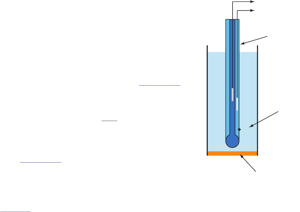
667
Chapter 11 Electrochemical Methods
an inner solution that contains an ion-selective electrode. e membrane is
permeable to the gaseous analyte, but impermeable to nonvolatile compo-
nents in the sample’s matrix. e gaseous analyte passes through the mem-
brane where it reacts with the inner solution, producing a species whose
concentration is monitored by the ion-selective electrode. For example, in
a CO
2
electrode, CO
2
diuses across the membrane where it reacts in the
inner solution to produce H
3
O
+
.
() () ()
()
aq la
qa
q
2CO HO HCOHO
22
3
3
?++
-+
11.12
e change in the activity of H
3
O
+
in the inner solution is monitored with
a pH electrode, for which the cell potential is given by equation 11.11. To
nd the relationship between the activity of H
3
O
+
in the inner solution
and the activity of CO
2
in the inner solution we rearrange the equilibrium
constant expression for reaction 11.12; thus
aK
a
a
HO a
HCO
CO
3
2
3
#=
+
-
11.13
where K
a
is the equilibrium constant. If the activity of
HCO
3
-
in the inter-
nal solution is suciently large, then its activity is not aected by the small
amount of CO
2
that passes through the membrane. Substituting equation
11.13 into equation 11.11 gives
.logEK a0 05916
cel
lC
O
2
=+
l
where K′ is a constant that includes the constant for the pH electrode, the
equilibrium constant for reaction 11.12 and the activity of
HCO
3
-
in the
inner solution.
Table 11.4 lists the properties of several gas-sensing electrodes. e
composition of the inner solution changes with use, and both the inner so-
lution and the membrane must be replaced periodically. Gas-sensing elec-
trodes are stored in a solution similar to the internal solution to minimize
their exposure to atmospheric gases.
PoTenTiomeTric Biosensors
e approach for developing gas-sensing electrodes can be modied to cre-
ate potentiometric electrodes that respond to a biochemically important
species. e most common class of potentiometric biosensors are
, in which we trap or immobilize an enzyme at the surface of
a potentiometric electrode. e analyte’s reaction with the enzyme pro-
duces a product whose concentration is monitored by the potentiometric
electrode. Potentiometric biosensors also have been designed around other
biologically active species, including antibodies, bacterial particles, tissues,
and hormone receptors.
One example of an enzyme electrode is the urea electrode, which is
based on the catalytic hydrolysis of urea by urease
() () () ()aq laqaqCO(NH) 2H O2NH CO
22 2
43
?++
+-
Figure 11.19 Schematic diagram of a
gas-sensing membrane electrode.
to meter
gas permeable
membrane
inner
solution
ISE

668
Analytical Chemistry 2.1
Figure 11.20 shows one version of the urea electrode, which modies a gas-
sensing NH
3
electrode by adding a dialysis membrane that traps a pH 7.0
buered solution of urease between the dialysis membrane and the gas per-
meable membrane.
4
When immersed in the sample, urea diuses through
the dialysis membrane where it reacts with the enzyme urease to form the
ammonium ion,
NH
4
+
, which
is in equilibrium with NH
3
.
() () () ()aq laqaqNH HO HO NH
4
23 3
?++
++
4 (a) Papastathopoulos, D. S.; Rechnitz, G. A. Anal. Chim. Acta 1975, 79, 17–26; (b) Riechel, T.
L. J. Chem. Educ. 1984, 61, 640–642.
Table 11.4 Representative Examples of Gas-Sensing Electrodes
analyte inner solution reaction in inner solution ion-selective electrode
CO
2
10 mM NaHCO
3
10 mM NaCl
() () () ()aq laqaq2CO HO HCOHO
22
3
3
?++
-+
glass pH ISE
HCN 10 mM KAg(CN)
2
() () () ()aq laqaqHCNHOCNHO
23
?++
-+
Ag
2
S solid-state ISE
HF 1 M H
3
O
+
() () () ()aq laqaqHF HO FHO
23
?++
-+
F
–
solid-state ISE
H
2
S pH 5 citrate buer
() () () ()aq laqaqHS HO HS HO
22 3
?++
-+
Ag
2
S solid-state ISE
NH
3
10 mM NH
4
Cl
0.1 M KNO
3
() () ()
()
aq la
qa
q
NH HO NH OH
32
4
?++
+-
glass pH ISE
NO
2
20 mM NaNO
2
0.1 M KNO
3
() ()
() ()
()
aq l
aq aq aq
2NO3HO
NO NO 2H O
22
32
3
?+
++
-- +
glass pH ISE
SO
2
1 mM NaHSO
3
pH 5
() () () ()aq laqaqSO 2H OHSO HO
22
3
3
?++
-+
glass pH ISE
Source: Cammann, K. Working With Ion-Selective Electrodes, Springer-Verlag: Berlin, 1977.
An NH
3
electrode, as shown in Table
11.4, uses a gas-permeable membrane and
a glass pH electrode. e NH
3
diuses
across the membrane where it changes the
pH of the internal solution.
Figure 11.20 Schematic diagram showing an enzyme-based po-
tentiometric biosensor for urea. A solution of the enzyme ure-
ase is trapped between a dialysis membrane and a gas permeable
membrane. Urea diuses across the dialysis membrane and reacts
with urease, producing NH
3
that diuses across the gas permeable
membrane. e resulting change in the internal solution’s pH is
measured with the pH electrode.
to meter
gas permeable
membrane
inner
solution
pH electrode
dialysis
membrane
urease
soluiton

669
Chapter 11 Electrochemical Methods
e NH
3
, in turn, diuses through the gas permeable membrane where a
pH electrode measures the resulting change in pH. e electrode’s response
to the concentration of urea is
.logEK a0 05916
cell urea
=-
11.14
Another version of the urea electrode (Figure 11.21) immobilizes the en-
zyme urease in a polymer membrane formed directly on the tip of a glass
pH electrode.
5
In this case the response of the electrode is
KapH
urea
=
11.15
Few potentiometric biosensors are available commercially. As shown in
Figure 11.20 and Figure 11.21, however, it is possible to convert an ion-
selective electrode or a gas-sensing electrode into a biosensor. Several rep-
resentative examples are described in Table 11.5, and additional examples
can be found in this chapter’s additional resources.
11B.5 Quantitative Applications
e potentiometric determination of an analyte’s concentration is one of
the most common quantitative analytical techniques. Perhaps the most
frequent analytical measurement is the determination of a solution’s pH, a
measurement we will consider in more detail later in this section. Other ar-
eas where potentiometry is important are clinical chemistry, environmental
chemistry, and potentiometric titrations. Before we consider representative
applications, however, we need to examine more closely the relationship
between cell potential and the analyte’s concentration and methods for
standardizing potentiometric measurements.
5 Tor, R.; Freeman, A. Anal. Chem. 1986, 58, 1042–1046.
Figure 11.21 Schematic diagram of an enzyme-based poten-
tiometric biosensor for urea in which urease is immobilized in
a polymer membrane coated onto the pH-sensitive glass mem-
brane of a pH electrode.
to meter
0.1 M HCl
porous wick
Ag/AgCl reference
electrode (internal)
Ag/AgCl reference
electrode (sample)
pH-sensitive
glass membrane
ureasae immoblized
in polymer membrane
Problem 11.7 asks you to show that equa-
tion 11.14 is correct.
Problem 11.8 asks you to explain the dif-
ference between equation 11.14 and equa-
tion 11.15.

670
Analytical Chemistry 2.1
acTiviTy and concenTraTion
e Nernst equation relates the cell potential to the analyte’s activity. For
example, the Nernst equation for a metallic electrode of the rst kind is
.
logEK
n
a
0 05916
Mcell
n
=+
+
11.16
where a
M
n+ is the metal ion’s activity. When we use a potentiometric elec-
trode, however, our goal is to determine the analyte’s concentration. As we
learned in Chapter 6, an ion’s activity is the product of its concentration,
[M
n+
], and a matrix-dependent activity coecient, c
M
n+.
[]aM
M
n
M
nn
c=
+
++
11.17
Substituting equation 11.17 into equation 11.16 and rearranging, gives
..
[]
lo
gl
ogEK
nn
M
0 05916 0 05916
M
n
cell
n
c=+ +
+
+
11.18
We can solve equation 11.18 for the metal ion’s concentration if we know
the value for its activity coecient. Unfortunately, if we do not know the
exact ionic composition of the sample’s matrix—which is the usual situ-
ation—then we cannot calculate the value of c
M
n+. ere is a solution to
this dilemma. If we design our system so that the standards and the samples
have an identical matrix, then the value of c
M
n+ remains constant and equa-
tion 11.18 simplies to
.
[]
logEK
n
M
0 05916
n
cell
=+
+
l
where K′ includes the activity coecient.
Table 11.5 Representative Examples of Potentiometric Biosensors
a
analyte biologically active phase
b
substance
determined
5′-adenosinemonophosphate (5′-AMP)
AMP-deaminase (E) NH
3
-arginine arginine and urease (E) NH
3
asparagine asparaginase (E)
NH
4
+
-cysteine Proteus morganii (B) H
2
S
-glutamate yellow squash (T) CO
2
-glutamine Sarcina ava (B) NH
3
oxalate oxalate decarboxylas (E) CO
2
penicillin pencillinase (E) H
3
O
+
-phenylalanine -amino acid oxidase/horseradish peroxidase (E) I
–
sugars bacteria from dental plaque (B) H
3
O
+
urea urease (E) NH
3
or H
3
O
+
a
Source: Complied from Cammann, K. Working With Ion-Selective Electrodes, Springer-Verlag: Berlin, 1977 and Lunte, C. E.; Heineman, W. R.
“Electrochemical techniques in Bioanalysis,” in Steckham, E. ed. Topics in Current Chemistry, Vol. 143, Springer-Verlag: Berlin, 1988, p.8.
b
Abbreviations: E = enzyme; B = bacterial particle; T = tissue.

671
Chapter 11 Electrochemical Methods
quanTiTaTive analysis usinG exTernal sTandards
Before we can determine the concentration of analyte in a sample, we must
standardize the electrode. If the electrode’s response obeys the Nernst equa-
tion, then we can determine the constant K using a single external standard.
Because a small deviation from the ideal slope of ±RT/nF or ±RT/zF is
not unexpected, we usually use two or more external standards.
In the absence of interferents, a calibration curve of E
cell
versus loga
A
,
where A is the analyte, is a straight-line. A plot of E
cell
versus log[A], how-
ever, may show curvature at higher concentrations of analyte as a result of
a matrix-dependent change in the analyte’s activity coecient. To maintain
a consistent matrix we add a high concentration of an inert electrolyte to
all samples and standards. If the concentration of added electrolyte is su-
cient, then the dierence between the sample’s matrix and the matrix of the
standards will not aect the ionic strength and the activity coecient essen-
tially remains constant. e inert electrolyte added to the sample and the
standards is called a (TISAB).
Example 11.8
e concentration of Ca
2+
in a water sample is determined using the
method of external standards. e ionic strength of the samples and the
standards is maintained at a nearly constant level by making each solution
0.5 M in KNO
3
. e measured cell potentials for the external standards
are shown in the following table.
[Ca
2+
] (M) E
cell
(V)
1.00�10
–5
–0.125
5.00�10
–5
–0.103
1.00�10
–4
–0.093
5.00�10
–4
–0.072
1.00�10
–3
–0.065
5.00�10
–3
–0.043
1.00�10
–2
–0.033
What is the concentration of Ca
2+
in a water sample if its cell potential is
found to be –0.084 V?
Solution
Linear regression gives the calibration curve in Figure 11.22, with an equa-
tion of
..[]logE 0 027 0 0303 Ca
2
cell
=+
+
Substituting the sample’s cell potential gives the concentration of Ca
2+
as 2.17�10
–4
M. Note that the slope of the calibration curve, which is
To review the use of external standards, see
Section 5C.2.
Figure 11.22 Calibration curve for the
data in Example 11.8.
-5.0 -4.5 -4.0 -3.5 -3.0 -2.5 -2.0
-0.14
-0.12
-0.10
-0.08
-0.06
-0.04
-0.02
log[Ca
2+
]
E
cell

672
Analytical Chemistry 2.1
0.0303, is slightly larger than its ideal value of 0.05916/2 = 0.02958; this
is not unusual and is one reason for using multiple standards.
quanTiTaTive analysis usinG The meThod oF sTandard addiTions
Another approach to calibrating a potentiometric electrode is the method
of standard additions. First, we transfer a sample with a volume of V
samp
and an analyte concentration of C
samp
into a beaker and measure the poten-
tial, (E
cell
)
samp
. Next, we make a standard addition by adding to the sample
a small volume, V
std
, of a standard that contains a known concentration
of analyte, C
std
, and measure the potential, (E
cell
)
std
. If V
std
is signicantly
smaller than V
samp
, then we can safely ignore the change in the sample’s
matrix and assume that the analyte’s activity coecient is constant. Ex-
ample 11.9 demonstrates how we can use a one-point standard addition to
determine the concentration of analyte in a sample.
Example 11.9
e concentration of Ca
2+
in a sample of sea water is determined using a
Ca ion-selective electrode and a one-point standard addition. A 10.00-mL
sample is transferred to a 100-mL volumetric ask and diluted to volume.
A 50.00-mL aliquot of the sample is placed in a beaker with the Ca ISE
and a reference electrode, and the potential is measured as –0.05290 V.
After adding a 1.00-mL aliquot of a 5.00 � 10
–2
M standard solution of
Ca
2+
the potential is –0.04417 V. What is the concentration of Ca
2+
in
the sample of sea water?
Solution
To begin, we write the Nernst equation before and after adding the stan-
dard addition. e cell potential for the sample is
()
.
logEK C
2
0 05916
cell samp samp
=+
and that following the standard addition is
()
.
logEK
V
V
C
V
V
C
2
0 05916
cell std
tot
samp
samp
tot
std
std
=+ +
&
0
where V
tot
is the total volume (V
samp
+ V
std
) after the standard addition.
Subtracting the rst equation from the second equation gives
() ()
..
lo
gl
og
EE E
V
V
C
V
V
CC
2
0 05916
2
0 05916
cell cell stdcellsamp
tot
samp
samp
tot
std
st
ds
amp
3 =- =
+-
&
0
Rearranging this equation leaves us with
.
log
E
V
V
VC
VC
0 05916
2
cell
tot
samp
totsamp
stdstd
3
=+
'
1
Substituting known values for DE, V
samp
, V
std
, V
tot
and C
std
,
To review the method of standard addi-
tions, see Section 5C.3.
One reason that it is not unusual to nd
that the experimental slope deviates from
its ideal value of 0.05916/n is that this
ideal value assumes that the temperature
is 25°C.

673
Chapter 11 Electrochemical Methods
.
{. (. )}
.
.
(. )
(. )(
.)
log
C
0 05916
20044 0050
51 00
50 00
51 00
100500 10
17 29
mL
mL
mL
mL M
2
samp
#
#
---
=
+
-
'
1
..
.
log
C
0 2951 0 9804
9 804 10
4
samp
#
=+
-
'
1
and taking the inverse log of both sides gives
..
.
C
1
973 0 9804
9 804 10
4
samp
#
=+
-
Finally, solving for C
samp
gives the concentration of Ca
2+
as 9.88 � 10
–4
M. Because we diluted the original sample of seawater by a factor of 10, the
concentration of Ca
2+
in the seawater sample is 9.88 � 10
–3
M.
Free ions versus comPlexed ions
Most potentiometric electrodes are selective toward the free, uncomplexed
form of the analyte, and do not respond to any of the analyte’s complexed
forms. is selectivity provides potentiometric electrodes with a signicant
advantage over other quantitative methods of analysis if we need to de-
termine the concentration of free ions. For example, calcium is present in
urine both as free Ca
2+
ions and as protein-bound Ca
2+
ions. If we analyze
a urine sample using atomic absorption spectroscopy, the signal is propor-
tional to the total concentration of Ca
2+
because both free and bound
calcium are atomized. Analyzing urine with a Ca
2+
ISE, however, gives a
signal that is a function of only free Ca
2+
ions because the protein-bound
Ca
2+
can not interact with the electrode’s membrane.
Representative Method 11.1
Determination of Fluoride in Toothpaste
Description of the MethoD
e concentration of uoride in toothpastes that contains soluble F
–
is
determined with a F
–
ion-selective electrode using a calibration curve pre-
pared with external standards. Although the F
–
ISE is very selective (only
OH
–
with a K
F
–
/OH
– of 0.1 is a signicant interferent), Fe
3+
and Al
3+
interfere with the analysis because they form soluble uoride complexes
that do not interact with the ion-selective electrode’s membrane. is
interference is minimized by reacting any Fe
3+
and Al
3+
with a suitable
complexing agent.
proceDure
Prepare 1 L of a standard solution of 1.00% w/v SnF
2
and transfer it to
a plastic bottle for storage. Using this solution, prepare 100 mL each of
e best way to appreciate the theoretical
and the practical details discussed in this
section is to carefully examine a typical
analytical method. Although each method
is unique, the following description of the
determination of F
–
in toothpaste pro-
vides an instructive example of a typical
procedure. e description here is based
on Kennedy, J. H. Analytical Chemistry—
Practice, Harcourt Brace Jaovanovich: San
Diego, 1984, p. 117–118.
Problem 11.14 provides some actual data
for the determination of uoride in tooth-
paste.

674
Analytical Chemistry 2.1
standards that contain 0.32%, 0.36%, 0.40%, 0.44% and 0.48% w/v
SnF
2
, adding 400 mg of malic acid to each solution as a stabilizer. Transfer
the standards to plastic bottles for storage. Prepare a total ionic strength
adjustment buer (TISAB) by mixing 500 mL of water, 57 mL of gla-
cial acetic acid, 58 g of NaCl, and 4 g of disodium DCTA (trans-1,2-
cyclohexanetetraacetic acid) in a 1-L beaker, stirring until dissolved. Cool
the beaker in a water bath and add 5 M NaOH until the pH is between
5–5.5. Transfer the contents of the beaker to a 1-L volumetric ask and
dilute to volume. Prepare each external standard by placing approximately
1 g of a uoride-free toothpaste, 30 mL of distilled water, and 1.00 mL
of standard into a 50-mL plastic beaker and mix vigorously for two min
with a stir bar. Quantitatively transfer the resulting suspension to a 100-
mL volumetric ask along with 50 mL of TISAB and dilute to volume
with distilled water. Store the entire external standard in a 250-mL plastic
beaker until you are ready to measure the potential. Prepare toothpaste
samples by obtaining an approximately 1-g portion and treating in the
same manner as the standards. Measure the cell potential for the exter-
nal standards and the samples using a F
–
ion-selective electrode and an
appropriate reference electrode. When measuring the potential, stir the
solution and allow two to three minutes to reach a stable potential. Report
the concentration of F
–
in the toothpaste %w/w SnF
2
.
Questions
1. e total ionic strength adjustment buer serves several purposes in
this procedure. Identify these purposes.
e composition of the TISAB has three purposes:
(a) e high concentration of NaCl (the nal solutions are approxi-
mately 1 M NaCl) ensures that the ionic strength of each exter-
nal standard and each sample is essentially identical. Because the
activity coecient for uoride is the same in all solutions, we can
write the Nernst equation in terms of uoride’s concentration
instead of its activity.
(b) e combination of glacial acetic acid and NaOH creates an acetic
acid/acetate buer of pH 5–5.5. As shown in Figure 11.23, the
pH of this buer is high enough to ensure that the predominate
form of uoride is F
–
instead of HF. is pH also is sucient-
ly acidic that it avoids an interference from OH
–
(see Example
11.8).
(c) DCTA is added as a complexing agent for Fe
3+
or Al
3+
, prevent-
ing the formation of
FeF
6
3-
or
AlF
6
3-
.
2. Why is a uoride-free toothpaste added to the standard solutions?
Adding a uoride-free toothpaste protects against any unaccounted
for matrix eects that might inuence the ion-selective electrode’s
Figure 11.23 Ladder diagram for
HF/F
–
. Maintaining a pH greater
than 4.2 ensures that the only sig-
nicant form of uoride is F
–
.
more acidic
more basic
pH
pK
a
= 3.17
HF
F
–
4.17
2.17
method’s
pH range

675
Chapter 11 Electrochemical Methods
measuremenT oF Ph
With the availability of inexpensive glass pH electrodes and pH meters, the
determination of pH is one of the most common quantitative analytical
measurements. e potentiometric determination of pH, however, is not
without complications, several of which we discuss in this section.
One complication is confusion over the meaning of pH.
6
e conven-
tional denition of pH in most general chemistry textbooks is
[]logpH H=-
+
11.19
As we now know, pH actually is a measure of the activity of H
+
.
log apH
H
=-
+
11.20
Equation 11.19 only approximates the true pH. If we calculate the pH of
0.1 M HCl using equation 11.19, we obtain a value of 1.00; the solution’s
actual pH, as dened by equation 11.20, is 1.1.
7
e activity and the con-
centration of H
+
are not the same in 0.1 M HCl because the activity coef-
cient for H
+
is not 1.00 in this matrix. Figure 11.24 shows a more colorful
demonstration of the dierence between activity and concentration.
A second complication in measuring pH is the uncertainty in the re-
lationship between potential and activity. For a glass membrane electrode,
the cell potential, (E
cell
)
samp
, for a sample of unknown pH is
()
.
lnEK
F
RT
a
K
F
RT
1
2 303
pH
cell samp
H
samp
=- =-
+
11.21
where K includes the potential of the reference electrode, the asymmetry
potential of the glass membrane, and any junction potentials in the electro-
chemical cell. All the contributions to K are subject to uncertainty, and may
change from day-to-day, as well as from electrode-to-electrode. For this
reason, before using a pH electrode we calibrate it using a standard buer
of known pH. e cell potential for the standard, (E
cell
)
std
, is
6 Kristensen, H. B.; Saloman, A.; Kokholm, G. Anal. Chem. 1991, 63, 885A–891A.
7 Hawkes, S. J. J. Chem. Educ. 1994, 71, 747–749.
response. is assumes, of course, that the matrices of the two tooth-
pastes are otherwise similar.
3. e procedure species that the standards and the sample should be
stored in plastic containers. Why is it a bad idea to store the solutions
in glass containers?
e uoride ion is capable of reacting with glass to form SiF
4
.
4. Suppose your calibration curve has a slope of –57.98 mV for each
10-fold change in the concentration of F
–
. e ideal slope from the
Nernst equation is –59.16 mV per 10-fold change in concentration.
What eect does this have on the quantitative analysis for uoride in
toothpaste?
No eect at all! is is why we prepare a calibration curve using mul-
tiple standards.
Try this experiment—nd several general
chemistry textbooks and look up pH in
each textbook’s index. Turn to the ap-
propriate pages and see how it is dened.
Next, look up activity or activity coecient
in each textbook’s index and see if these
terms are indexed.

676
Analytical Chemistry 2.1
()
.
EK
F
RT2 303
pH
cell st
ds
td
=-
11.22
where pH
std
is the standard’s pH. Subtracting equation 11.22 from equa-
tion 11.21 and solving for pH
samp
gives
.
() ()
RT
EEF
2 303
pH pH
samp std
cell samp cell std
=-
-
"
,
11.23
which is the operational denition of pH adopted by the International
Union of Pure and Applied Chemistry.
8
Calibrating a pH electrode presents a third complication because we
need a standard with an accurately known activity for H
+
. Table 11.6 pro-
vides pH values for several primary standard buer solutions accepted by
the National Institute of Standards and Technology.
To standardize a pH electrode using two buers, choose one near a
pH of 7 and one that is more acidic or basic depending on your sample’s
expected pH. Rinse your pH electrode in deionized water, blot it dry with a
laboratory wipe, and place it in the buer with the pH closest to 7. Swirl the
pH electrode and allow it to equilibrate until you obtain a stable reading.
Adjust the “Standardize” or “Calibrate” knob until the meter displays the
correct pH. Rinse and dry the electrode, and place it in the second buer.
After the electrode equilibrates, adjust the “Slope” or “Temperature” knob
until the meter displays the correct pH.
Some pH meters can compensate for a change in temperature. To use
this feature, place a temperature probe in the sample and connect it to the
pH meter. Adjust the “Temperature” knob to the solution’s temperature
and calibrate the pH meter using the “Calibrate” and “Slope” controls. As
you are using the pH electrode, the pH meter compensates for any change
in the sample’s temperature by adjusting the slope of the calibration curve
using a Nernstian response of 2.303RT/F.
8 Covington, A. K.; Bates, R. B.; Durst, R. A. Pure & Appl. Chem. 1985, 57, 531–542.
Figure 11.24 A demonstration of the dierence between activity and concentra-
tion using the indicator methyl green. e indicator is pale yellow in its acid form
(beaker a: 1.0 M HCl) and is blue in its base form (beaker d: H
2
O). In 10 mM
HCl the indicator is in its base form (beaker b: 20 mL of 10 mM HCl with 3 drops
of methyl green). Adding 20 mL of 5 M LiCl to this solution shifts the indica-
tor's color to green (beaker c); although the concentration of HCl is cut in half
to 5 mM, the activity of H
+
has increased as evidenced by the green color that is
intermediate between the indicator’s pale yellow, acid form and its blue, base form.
e demonstration shown here is adapted
from McCarty, C. G.; Vitz, E. “pH Para-
doxes: Demonstrating at It Is Not True
at pH ≡ –log[H
+
],” J. Chem. Educ.
2006, 83, 752–757. is paper provides
several additional demonstrations that il-
lustrate the dierence between concentra-
tion and activity.
e equations in this section assume that
the pH electrode is the cathode in a po-
tentiometric cell. In this case an increase
in pH corresponds to a decrease in the cell
potential. Many pH meters are designed
with the pH electrode as the anode, result-
ing in an increase in the cell potential for
higher pH values. e operational deni-
tion of pH in this case is
.
() ()
RT
EE
F
2 303
pH pH
samp std
cell samp cell std
=+
-
"
,
e dierence between this equation and
equation 11.23 does not aect the opera-
tion of a pH meter.

677
Chapter 11 Electrochemical Methods
clinical aPPlicaTions
Because of their selectivity for analytes in complex matricies, ion-selective
electrodes are important sensors for clinical samples. e most common an-
alytes are electrolytes, such as Na
+
, K
+
, Ca
2+
, H
+
, and Cl
–
, and dissolved
gases such as CO
2
. For extracellular uids, such as blood and urine, the
analysis can be made in vitro. An in situ analysis, however, requires a much
smaller electrode that we can insert directly into a cell. Liquid-based mem-
brane microelectrodes with tip diameters smaller than 1 µm are constructed
by heating and drawing out a hard-glass capillary tube with an initial diam-
eter of approximately 1–2 mm (Figure 11.25). e microelectrode’s tip is
made hydrophobic by dipping into a solution of dichlorodimethyl silane,
and an inner solution appropriate for the analyte and a Ag/AgCl wire refer-
ence electrode are placed within the microelectrode. e microelectrode is
dipped into a solution of the liquid complexing agent, which through cap-
illary action draws a small volume of the liquid complexing agent into the
tip. Potentiometric microelectrodes have been developed for a number of
clinically important analytes, including H
+
, K
+
, Na
+
, Ca
2+
, Cl
–
, and I
–
.
9
environmenTal aPPlicaTions
Although ion-selective electrodes are used in environmental analysis, their
application is not as widespread as in clinical analysis. Although standard
potentiometric methods are available for the analysis of CN
–
, F
–
, NH
3
,
and
NO
3
-
in water and wastewater, other analytical methods generally pro-
9 Bakker, E.; Pretsch, E. Trends Anal. Chem. 2008, 27, 612–618.
Table 11.6 pH Values for Selected NIST Primary Standard Buers
temp
(
o
C)
saturated
(at 25
o
C)
KHC
4
H
4
O
7
(tartrate)
0.05 m
KH
2
C
6
H
5
O
7
(citrate)
0.05 m
KHC
8
H
4
O
4
(phthalate)
0.025 m
KH
2
PO
4
,
0.025 m
Na
2
HPO
4
0.008 695
m KH
2
PO
4
,
0.030 43 m
Na
2
HPO
4
0.01 m
Na
4
B
4
O
7
0.025 m
NaHCO
3
,
0.025 m
Na
2
CO
3
0 — 3.863 4.003 6.984 7.534 9.464 10.317
5 — 3.840 3.999 6.951 7.500 9.395 10.245
10 — 3.820 3.998 6.923 7.472 9.332 10.179
15 — 3.802 3.999 6.900 7.448 9.276 10.118
20 — 3.788 4.002 6.881 7.429 9.225 10.062
25 3.557 3.776 4.008 6.865 7.413 9.180 10.012
30 3.552 3.766 4.015 6.854 7.400 9.139 9.966
35 3.549 3.759 4.024 6.844 7.389 9.012 9.925
40 3.547 3.753 4.035 6.838 7.380 9.068 9.889
45 3/547 3.750 4.047 6.834 7.373 9.038 9.856
50 3.549 3.749 4.060 6.833 7.367 9.011 9.828
Source: Values taken from Bates, R. G. Determination of pH: eory and Practice, 2nd ed. Wiley: New York, 1973. See also Buck, R. P., et. al.
“Measurement of pH. Denition, Standards, and Procedures,” Pure. Appl. Chem. 2002, 74, 2169–2200.
Figure 11.25 Schematic diagram of a
liquid-based ion-selective microelec-
trode.
<1µm
to meter
inner
solution
Ag/AgCl
reference electrode

678
Analytical Chemistry 2.1
vide better detection limits. One potential advantage of an ion-selective
electrode is the ability to incorporate it into a ow cell for the continuous
monitoring of wastewater streams.
PoTenTiomeTric TiTraTions
One method for determining the equivalence point of an acid–base titra-
tion is to use a pH electrode to monitor the change in pH during the titra-
tion. A potentiometric determination of the equivalence point is possible
for acid–base, complexation, redox, and precipitation titrations, as well as
for titrations in aqueous and nonaqueous solvents. Acid–base, complex-
ation, and precipitation potentiometric titrations usually are monitored
with an ion-selective electrode that responds the analyte, although an elec-
trode that responds to the titrant or a reaction product also can be used.
A redox electrode, such as a Pt wire, and a reference electrode are used for
potentiometric redox titrations. More details about potentiometric titra-
tions are found in Chapter 9.
11B.6 Evaluation
scale oF oPeraTion
e working range for most ion-selective electrodes is from a maximum
concentration of 0.1–1 M to a minimum concentration of 10
–5
–10
–11
M.
10
is broad working range extends from major analytes to ultratrace analytes,
and is signicantly greater than many other analytical techniques. To use
a conventional ion-selective electrode we need a minimum sample volume
of several mL (a macro sample). Microelectrodes, such as the one shown in
Figure 11.25, are used with an ultramicro sample, although care is needed
to ensure that the sample is representative of the original sample.
accuracy
e accuracy of a potentiometric analysis is limited by the error in measur-
ing E
cell
. Several factors contribute to this measurement error, including the
contribution to the potential from interfering ions, the nite current that
passes through the cell while we measure the potential, dierences between
the analyte’s activity coecient in the samples and the standard solutions,
and junction potentials. We can limit the eect of an interfering ion by in-
cluding a separation step before the potentiometric analysis. Modern high
impedance potentiometers minimize the amount of current that passes
through the electrochemical cell. Finally, we can minimize the errors due to
activity coecients and junction potentials by matching the matrix of the
standards to that of the sample. Even in the best circumstances, however, a
10 (a) Bakker, E.; Pretsch, E. Anal. Chem. 2002, 74, 420A–426A; (b) Bakker, E.; Pretsch, E. Trends
Anal. Chem. 2005, 24, 199–207.
See Figure 3.5 to review the meaning of
major and ultratrace analytes, and the
meaning of macro and ultramicro sam-
ples.

679
Chapter 11 Electrochemical Methods
dierence of approximately ±1mV for samples with equal concentrations
of analyte is not unusual.
We can evaluate the eect of uncertainty on the accuracy of a poten-
tiometric measurement by using a propagation of uncertainty. For a mem-
brane ion-selective electrode the general expression for potential is
[]
lnEK
zF
RT
A
cell
=+
where z is the analyte’s, A, charge. From Table 4.10 in Chapter 4, the un-
certainty in the cell potential, DE
cell
is
[]
[]
E
zF
RT
A
A
cell
3#
3
=
Rearranging and multiplying through by 100 gives the percent relative error
in concentration as
[]
[]
/RT zF
E
100 100%relativeerror
A
A
cell
3
#
3
#==
11.24
e relative error in concentration, therefore, is a function of the measure-
ment error for the electrode’s potential, DE
cell
, and the analyte’s charge.
Table 11.7 provides representative values for ions with charges of ±1 and
±2 at a temperature of 25
o
C. Accuracies of 1–5% for monovalent ions
and 2–10% for divalent ions are typical. Although equation 11.24 applies
to membrane electrodes, we can use if for a metallic electrode by replacing
z with n.
Precision
Precision in potentiometry is limited by variations in temperature and the
sensitivity of the potentiometer. Under most conditions—and when using
a simple, general-purpose potentiometer—we can measure the potential
with a repeatability of ±0.1 mV. Using Table 11.7, this corresponds to an
uncertainty of ±0.4% for monovalent analytes and ±0.8% for divalent
Table 11.7 Relationship Between The Uncertainty in
Measuring E
cell
and the Relative Error in the
Analyte’s Concentration
% relative error in concentration
DE
cell
(±mV) z = ±1 z = ±2
0.1
±0.4 ±0.8
0.5
±1.9 ±3.9
1.0
±3.9 ±7.8
1.5
±5.8 ±11.1
2.0
±7.8 ±15.6

680
Analytical Chemistry 2.1
analytes. e reproducibility of potentiometric measurements is about a
factor of ten poorer.
sensiTiviTy
e sensitivity of a potentiometric analysis is determined by the term RT/nF
or RT/zF in the Nernst equation. Sensitivity is best for smaller values of n
or z.
selecTiviTy
As described earlier, most ion-selective electrodes respond to more than one
analyte; the selectivity for the analyte, however, often is signicantly greater
than the sensitivity for the interfering ions. e manufacturer of an ion-
selective usually provides an ISE’s selectivity coecients, which allows us to
determine whether a potentiometric analysis is feasible for a given sample.
Time, cosT, and equiPmenT
In comparison to other techniques, potentiometry provides a rapid, rel-
atively low-cost means for analyzing samples. e limiting factor when
analyzing a large number of samples is the need to rinse the electrode be-
tween samples. e use of inexpensive, disposable ion-selective electrodes
can increase a lab’s sample throughput. Figure 11.26 shows one example
of a disposable ISE for Ag
+
.
11
Commercial instruments for measuring pH
or potential are available in a variety of price ranges, and includes portable
models for use in the eld.
11 Tymecki, L.; Zwierkowska, E.; Głąb, S.; Koncki, R. Sens. Actuators B 2003, 96, 482–488.
Figure 11.26 Schematic diagram of a disposable
ion-selective electrode created by screen-printing.
In (a) a thin lm of conducting silver is printed on
a polyester substrate and a lm of Ag
2
S overlaid
near the bottom. In (b) an insulation layer with
a small opening is layered on top exposes a por-
tion of the Ag
2
S membrane that is immersed in the
sample. e top of the polyester substrate remains
uncoated, which allows us to connect the electrode
to a potentiometer through the Ag lm. e small
inset shows the electrode’s actual size.
polyester
substrate
Ag
Ag
2
S
4 mm
24 mm
1.5 mm x 1.5 mm
opening
Ag
polyester
substrate
insulation
layer
(a)
(b)

681
Chapter 11 Electrochemical Methods
11C Coulometric Methods
In a potentiometric method of analysis we determine an analyte’s concen-
tration by measuring the potential of an electrochemical cell under static
conditions in which no current ows and the concentrations of species
in the electrochemical cell remain xed. Dynamic techniques, in which
current passes through the electrochemical cell and concentrations change,
also are important electrochemical methods of analysis. In this section we
consider coulometry. Voltammetry and amperometry are covered in sec-
tion 11D.
C is based on an exhaustive electrolysis of the analyte. By
exhaustive we mean that the analyte is oxidized or reduced completely at
the working electrode, or that it reacts completely with a reagent generated
at the working electrode. ere are two forms of coulometry: -
, in which we apply a constant potential to the
electrochemical cell, and - , in which
we pass a constant current through the electrochemical cell.
During an electrolysis, the total charge, Q, in coulombs, that passes
through the electrochemical cell is proportional to the absolute amount of
analyte by ’
QnFN
A
=
11.25
where n is the number of electrons per mole of analyte, F is Faraday’s
constant (96 487 C mol
–1
), and N
A
is the moles of analyte. A coulomb is
equivalent to an A
.
sec; thus, for a constant current, i, the total charge is
Qit
e
=
11.26
where t
e
is the electrolysis time. If the current varies with time, as it does in
controlled-potential coulometry, then the total charge is
()
Qi
tdt
t
0
e
=
#
11.27
In coulometry, we monitor current as a function of time and use either
equation 11.26 or equation 11.27 to calculate Q. Knowing the total charge,
we then use equation 11.25 to determine the moles of analyte. To obtain
an accurate value for N
A
, all the current must oxidize or reduce the analyte;
that is, coulometry requires 100% or an accurate
measurement of the current eciency using a standard.
11C.1 Controlled-Potential Coulometry
e easiest way to ensure 100% current eciency is to hold the working
electrode at a constant potential where the analyte is oxidized or reduced
completely and where no potential interfering species are oxidized or re-
duced. As electrolysis progresses, the analyte’s concentration and the current
decrease. e resulting current-versus-time prole for controlled-potential
coulometry is shown in Figure 11.27. Integrating the area under the curve
Current eciency is the percentage of
current that actually leads to the analyte’s
oxidation or reduction.

682
Analytical Chemistry 2.1
(equation 11.27) from t = 0 to t = t
e
gives the total charge. In this section
we consider the experimental parameters and instrumentation needed to
develop a controlled-potential coulometric method of analysis.
selecTinG a consTanT PoTenTial
To understand how an appropriate potential for the working electrode is
selected, let’s develop a constant-potential coulometric method for Cu
2+
based on its reduction to copper metal at a Pt working electrode.
()
()e
aq s
Cu 2Cu
2
?+
+-
11.28
Figure 11.28 shows a ladder diagram for an aqueous solution of Cu
2+
.
From the ladder diagram we know that reaction 11.28 is favored when the
working electrode’s potential is more negative than +0.342 V versus the
standard hydrogen electrode. To ensure a 100% current eciency, however,
the potential must be suciently more positive than +0.000 V so that the
reduction of H
3
O
+
to H
2
does not contribute signicantly to the total
current owing through the electrochemical cell.
We can use the Nernst equation for reaction 11.28 to estimate the
minimum potential for quantitatively reducing Cu
2+
.
.
[]
logEE
2
0 05916
1
Cu
Cu /Cu
o
2
2
=-
+
+
11.29
If we dene a quantitative electrolysis as one in which we reduce 99.99%
of Cu
2+
to Cu, then the concentration of Cu
2+
at t
e
is
[] .[]0 0001Cu Cu
t 0
22
e
#=
++
11.30
where [Cu
2+
]
0
is the initial concentration of Cu
2+
in the sample. Substitut-
ing equation 11.30 into equation 11.29 allows us to calculate the desired
potential.
Figure 11.27 Current versus time for a controlled-poten-
tial coulometric analysis. e measured current is shown
by the red curve. e integrated area under the curve,
shown in blue, is the total charge.
time
current
t = t
e
Qitdt
t
e
=
∫
()
0
Figure 11.28 Ladder diagram for an
aqueous solution of Cu
2+
showing
steps for the reductions of O
2
to H
2
O,
of Cu
2+
to Cu, and of H
3
O
+
to H
2
.
For each step, the oxidized species is in
blue and the reduced species is in red.
So why are we using the concentration
of Cu
2+
in equation 11.29 instead of
its activity? In potentiometry we use ac-
tivity because we use E
cell
to determine
the analyte’s concentration. Here we use
the Nernst equation to help us select an
appropriate potential. Once we iden-
tify a potential, we can adjust its value as
needed to ensure a quantitative reduction
of Cu
2+
. In addition, in coulometry the
analyte’s concentration is given by the to-
tal charge, not the applied potential.
E
E
o
H
3
O
+
/H
2
= +0.000 V
E
o
Cu
2+
/Cu
= +0.342 V
Cu
2+
more negative
more positive
E
o
O
2
/H
2
O
= +1.229 V
Cu
H
3
O
+
H
2
O
2
H
2
O

683
Chapter 11 Electrochemical Methods
.
.[]
logEE
2
0 05916
0 0001
1
Cu
Cu /Cu
o
2
2
#
=-
+
+
If the initial concentration of Cu
2+
is 1.00 � 10
–4
M, for example, then
the working electrode’s potential must be more negative than +0.105 V to
quantitatively reduce Cu
2+
to Cu. Note that at this potential H
3
O
+
is not
reduced to H
2
, maintaining 100% current eciency.
minimizinG elecTrolysis Time
In controlled-potential coulometry, as shown in Figure 11.27, the current
decreases over time. As a result, the rate of electrolysis—recall from Section
11A that current is a measure of rate—becomes slower and an exhaustive
electrolysis of the analyte may require a long time. Because time is an im-
portant consideration when designing an analytical method, we need to
consider the factors that aect the analysis time.
We can approximate the current’s change as a function of time in Figure
11.27 as an exponential decay; thus, the current at time t is
iie
t
kt
0
=
-
11.31
where i
0
is the current at t = 0 and k is a rate constant that is directly pro-
portional to the area of the working electrode and the rate of stirring, and
that is inversely proportional to the volume of solution. For an exhaustive
electrolysis in which we oxidize or reduce 99.99% of the analyte, the cur-
rent at the end of the analysis, t
e
, is
.ii0 0001
t 0
e
##
11.32
Substituting equation 11.32 into equation 11.31 and solving for t
e
gives
the minimum time for an exhaustive electrolysis as
ß(.)
.
lnt
kk
1
0 0001
921
e
#=- =
From this equation we see that a larger value for k reduces the analysis
time. For this reason we usually carry out a controlled-potential coulomet-
ric analysis in a small volume electrochemical cell, using an electrode with
a large surface area, and with a high stirring rate. A quantitative electrolysis
typically requires approximately 30–60 min, although shorter or longer
times are possible.
insTrumenTaTion
A three-electrode potentiostat is used to set the potential in controlled-
potential coulometry. e working electrodes is usually one of two types: a
cylindrical Pt electrode manufactured from platinum-gauze (Figure 11.29),
or a Hg pool electrode. e large overpotential for the reduction of H
3
O
+
at Hg makes it the electrode of choice for an analyte that requires a nega-
tive potential. For example, a potential more negative than –1 V versus the
SHE is feasible at a Hg electrode—but not at a Pt electrode—even in a very
acidic solution. Because mercury is easy to oxidize, it is less useful if we need
Many controlled-potential coulometric
methods for Cu
2+
use a potential that is
negative relative to the standard hydrogen
electrode—see, for example, Rechnitz, G.
A. Controlled-Potential Analysis, Macmil-
lan: New York, 1963, p.49.
Based on the ladder diagram in Figure
11.28 you might expect that applying a
potential <0.000 V will partially reduce
H
3
O
+
to H
2
, resulting in a current ef-
ciency that is less than 100%. e rea-
son we can use such a negative potential is
that the reaction rate for the reduction of
H
3
O
+
to H
2
is very slow at a Pt electrode.
is results in a signicant -
—the need to apply a potential more
positive or a more negative than that pre-
dicted by thermodynamics—which shifts
E
o
for the H
3
O
+
/H
2
redox couple to a
more negative value.
Problem 11.16 asks you to explain why
a larger surface area, a faster stirring rate,
and a smaller volume leads to a shorter
analysis time.
Figure 11.5 shows an example of a manual
three-electrode potentiostat. Although a
modern potentiostat uses very dierent
circuitry, you can use Figure 11.5 and the
accompanying discussion to understand
how we can use the three electrodes to set
the potential and to monitor the current.

684
Analytical Chemistry 2.1
to maintain a potential that is positive with respect to the SHE. Platinum is
the working electrode of choice when we need to apply a positive potential.
e auxiliary electrode, which often is a Pt wire, is separated by a salt
bridge from the analytical solution. is is necessary to prevent the elec-
trolysis products generated at the auxiliary electrode from reacting with
the analyte and interfering in the analysis. A saturated calomel or Ag/AgCl
electrode serves as the reference electrode.
e other essential need for controlled-potential coulometry is a means
for determining the total charge. One method is to monitor the current
as a function of time and determine the area under the curve, as shown in
Figure 11.27. Modern instruments use electronic integration to monitor
charge as a function of time. e total charge at the end of the electrolysis
is read directly from a digital readout.
elecTroGravimeTry
If the product of controlled-potential coulometry forms a deposit on the
working electrode, then we can use the change in the electrode’s mass as the
analytical signal. For example, if we apply a potential that reduces Cu
2+
to
Cu at a Pt working electrode, the dierence in the electrode’s mass before
and after electrolysis is a direct measurement of the amount of copper in
the sample. As we learned in Chapter 8, we call an analytical technique
that uses mass as a signal a gravimetric technique; thus, we call this -
.
11C.2 Controlled-Current Coulometry
A second approach to coulometry is to use a constant current in place of a
constant potential, which results in the current-versus-time prole shown
in Figure 11.30. Controlled-current coulometry has two advantages over
controlled-potential coulometry. First, the analysis time is shorter because
the current does not decrease over time. A typical analysis time for con-
trolled-current coulometry is less than 10 min, compared to approximately
30–60 min for controlled-potential coulometry. Second, because the total
charge simply is the product of current and time (equation 11.26), there is
no need to integrate the current-time curve in Figure 11.30.
Using a constant current presents us with two important experimental
problems. First, during electrolysis the analyte’s concentration—and, there-
fore, the current that results from its oxidation or reduction—decreases
continuously. To maintain a constant current we must allow the potential
to change until another oxidation reaction or reduction reaction occurs at
the working electrode. Unless we design the system carefully, this secondary
reaction results in a current eciency that is less than 100%. e second
problem is that we need a method to determine when the analyte's elec-
trolysis is complete. As shown in Figure 11.27, in a controlled-potential
coulometric analysis we know that electrolysis is complete when the current
Figure 11.29 Example of a cylindrical
Pt-gauze electrode used in controlled-
potential coulometry. e electrode
shown here has a diameter of 13 mm
and a height of 48 mm, and was fash-
ioned from Pt wire with a diameter
of approximately 0.15 mm. e elec-
trode’s surface has 360 openings/cm
2
and a total surface area of approxi-
mately 40 cm
2
.
Figure 11.30 Current versus time for a
controlled-current coulometric analy-
sis. e measured current is shown
by the red curve. e integrated area
under the curve, shown in blue, is the
total charge.
time
current
t = t
e
Q = it

685
Chapter 11 Electrochemical Methods
reaches zero, or when it reaches a constant background or residual current.
In a controlled-current coulometric analysis, however, current continues to
ow even when the analyte’s electrolysis is complete. A suitable method for
determining the reaction’s endpoint, t
e
, is needed.
mainTaininG currenT eFFiciency
To illustrate why a change in the working electrode’s potential may result
in a current eciency of less than 100%, let’s consider the coulometric
analysis for Fe
2+
based on its oxidation to Fe
3+
at a Pt working electrode
in 1 M H
2
SO
4
.
() () eaq aqFe Fe
23
? +
++-
Figure 11.31 shows the ladder diagram for this system. At the beginning of
the analysis, the potential of the working electrode remains nearly constant
at a level near its initial value. As the concentration of Fe
2+
decreases and
the concentration of Fe
3+
increases, the working electrode’s potential shifts
toward more positive values until the oxidation of H
2
O begins.
() () ()
e
lg aq
2H OO 4H 4
22
? ++
+-
Because a portion of the total current comes from the oxidation of H
2
O,
the current eciency for the analysis is less than 100% and we cannot use
equation 11.25 to determine the amount of Fe
2+
in the sample.
Although we cannot prevent the potential from drifting until another
species undergoes oxidation, we can maintain a 100% current eciency if
the product of that secondary oxidation reaction both rapidly and quantita-
tively reacts with the remaining Fe
2+
. To accomplish this we add an excess
of Ce
3+
to the analytical solution. As shown in Figure 11.32, when the
potential of the working electrode shifts to a more positive potential, Ce
3+
begins to oxidize to Ce
4+
() ()
e
aq aq
Ce Ce
34
?
+
++-
11.33
e Ce
4+
that forms at the working electrode rapidly mixes with the solu-
tion where it reacts with any available Fe
2+
.
() () () ()
aq aq aq aq
Ce Fe Ce Fe
4233
?++
++
++
11.34
Combining reaction 11.33 and reaction 11.34 shows that the net reaction
is the oxidation of Fe
2+
to Fe
3+
() () eaq aqFe Fe
23
? +
++-
which maintains a current eciency of 100%. A species used to maintain
100% current eciency is called a .
endPoinT deTerminaTion
Adding a mediator solves the problem of maintaining 100% current e-
ciency, but it does not solve the problem of determining when the analyte's
electrolysis is complete. Using the analysis for Fe
2+
in Figure 11.32, when
Figure 11.31 Ladder diagram for the
constant-current coulometric analysis
of Fe
2+
. e red arrow and text shows
how the potential drifts to more posi-
tive values, decreasing the current ef-
ciency.
E
E
o
H
3
O
+
/H
2
E
o
Fe
3+
/Fe
2+
= +0.68 V
Fe
3+
more negative
more positive
E
o
O
2
/H
2
O
Fe
2+
potential drifts
until H
2
O
undergoes oxidation
initial potential
Figure 11.32 Ladder diagram for the
constant-current coulometric analysis
of Fe
2+
in the presence of a Ce
3+
me-
diator. As the potential drifts to more
positive values, we eventually reach a
potential where Ce
3+
undergoes oxi-
dation. Because Ce
4+
, the product
of the oxidation of Ce
3+
, reacts with
Fe
2+
, we maintain current eciency.
E
E
o
H
3
O
+
/H
2
E
o
Fe
3+
/Fe
2+
= +0.68 V
Fe
3+
more negative
more positive
E
o
O
2
/H
2
O
Fe
2+
E
o
Ce
4+
/Ce
3+
= +1.44 V
Ce
4+
Ce
3+
Ce
4+
Fe
2+
Ce
3+
Fe
3+
++

686
Analytical Chemistry 2.1
the oxidation of Fe
2+
is complete current continues to ow from the oxi-
dation of Ce
3+
, and, eventually, the oxidation of H
2
O. What we need is a
signal that tells us when no more Fe
2+
is present in the solution.
For our purposes, it is convenient to treat a controlled-current coulo-
metric analysis as a reaction between the analyte, Fe
2+
, and the mediator,
Ce
3+
, as shown by reaction 11.34. is reaction is identical to a redox titra-
tion; thus, we can use the end points for a redox titration—visual indicators
and potentiometric or conductometric measurements—to signal the end of
a controlled-current coulometric analysis. For example, ferroin provides a
useful visual endpoint for the Ce
3+
mediated coulometric analysis for Fe
2+
,
changing color from red to blue when the electrolysis of Fe
2+
is complete.
insTrumenTaTion
Controlled-current coulometry normally is carried out using a two-elec-
trode galvanostat, which consists of a working electrode and a counter elec-
trode. e working electrode—often a simple Pt electrode—also is called
the generator electrode since it is where the mediator reacts to generate the
species that reacts with the analyte. If necessary, the counter electrode is
isolated from the analytical solution by a salt bridge or a porous frit to pre-
vent its electrolysis products from reacting with the analyte. Alternatively,
we can generate the oxidizing agent or the reducing agent externally, and
allow it to ow into the analytical solution. Figure 11.33 shows one simple
method for accomplishing this. A solution that contains the mediator ows
into a small-volume electrochemical cell with the products exiting through
separate tubes. Depending upon the analyte, the oxidizing agent or the re-
ducing reagent is delivered to the analytical solution. For example, we can
generate Ce
4+
using an aqueous solution of Ce
3+
, directing the Ce
4+
that
forms at the anode to our sample.
Reaction 11.34 is the same reaction we
used in Chapter 9 to develop our under-
standing of redox titrimetry.
See Figure 9.40 for the titration curve and
for ferroin's color change.
Figure 11.4 shows an example of a manual
galvanostat. Although a modern galvanos-
tat uses very dierent circuitry, you can use
Figure 11.4 and the accompanying discus-
sion to understand how we can use the
working electrode and the counter elec-
trode to control the current. Figure 11.4
includes an optional reference electrode,
but its presence or absence is not impor-
tant if we are not interested in monitoring
the working electrode’s potential.
anodecathode
mediator
solution
source of
reducing agent
source of
oxidizing agent
glass
wool
Figure 11.33 One example of a device for the ex-
ternal generation of oxidizing agents and reducing
agents for controlled-current coulometry. A solu-
tion containing the mediator ows into a small-vol-
ume electrochemical cell. e resulting oxidation
products, which form at the anode, ow to the right
and serve as an oxidizing agent. Reduction at the
cathode generates a reducing agent.

687
Chapter 11 Electrochemical Methods
ere are two other crucial needs for controlled-current coulometry:
an accurate clock for measuring the electrolysis time, t
e
, and a switch for
starting and stopping the electrolysis. An analog clock can record time to
the nearest ±0.01 s, but the need to stop and start the electrolysis as we ap-
proach the endpoint may result in an overall uncertainty of ±0.1 s. A digital
clock allows for a more accurate measurement of time, with an overall un-
certainty of ±1 ms. e switch must control both the current and the clock
so that we can make an accurate determination of the electrolysis time.
coulomeTric TiTraTions
A controlled-current coulometric method sometimes is called a -
because of its similarity to a conventional titration. For
example, in the controlled-current coulometric analysis for Fe
2+
using a
Ce
3+
mediator, the oxidation of Fe
2+
by Ce
4+
(reaction 11.34) is identical
to the reaction in a redox titration (reaction 9.15).
ere are other similarities between controlled-current coulometry and
titrimetry. If we combine equation 11.25 and equation 11.26 and solve for
the moles of analyte, N
A
, we obtain the following equation.
N
nF
i
t
Ae
#=
11.35
Compare equation 11.35 to the relationship between the moles of analyte,
N
A
, and the moles of titrant, N
T
, in a titration
NNMV
AT TT
#==
where M
T
and V
T
are the titrant’s molarity and the volume of titrant at the
end point. In constant-current coulometry, the current source is equiva-
lent to the titrant and the value of that current is analogous to the titrant’s
molarity. Electrolysis time is analogous to the volume of titrant, and t
e
is
equivalent to the a titration’s end point. Finally, the switch for starting and
stopping the electrolysis serves the same function as a buret’s stopcock.
11C.3 Quantitative Applications
Coulometry is used for the quantitative analysis of both inorganic and
organic analytes. Examples of controlled-potential and controlled-current
coulometric methods are discussed in the following two sections.
conTrolled-PoTenTial coulomeTry
e majority of controlled-potential coulometric analyses involve the de-
termination of inorganic cations and anions, including trace metals and
halides ions. Table 11.8 summarizes several of these methods.
e ability to control selectivity by adjusting the working electrode’s
potential makes controlled-potential coulometry particularly useful for the
analysis of alloys. For example, we can determine the composition of an
alloy that contains Ag, Bi, Cd, and Sb by dissolving the sample and plac-
For simplicity, we assume that the stoichi-
ometry between the analyte and titrant is
1:1. e assumption, however, is not im-
portant and does not eect our observa-
tion of the similarity between controlled-
current coulometry and a titration.

688
Analytical Chemistry 2.1
ing it in a matrix of 0.2 M H
2
SO
4
along with a Pt working electrode and
a Pt counter electrode. If we apply a constant potential of +0.40 V versus
the SCE, Ag(I) deposits on the electrode as Ag and the other metal ions
remain in solution. When electrolysis is complete, we use the total charge
to determine the amount of silver in the alloy. Next, we shift the work-
ing electrode’s potential to –0.08 V versus the SCE, depositing Bi on the
working electrode. When the coulometric analysis for bismuth is complete,
we determine antimony by shifting the working electrode’s potential to
–0.33 V versus the SCE, depositing Sb. Finally, we determine cadmium
following its electrodeposition on the working electrode at a potential of
–0.80 V versus the SCE.
We also can use controlled-potential coulometry for the quantitative
analysis of organic compounds, although the number of applications is
signicantly less than that for inorganic analytes. One example is the six-
electron reduction of a nitro group, –NO
2
, to a primary amine, –NH
2
, at
a mercury electrode. Solutions of picric acid—also known as 2,4,6-trini-
trophenol, or TNP, a close relative of TNT—is analyzed by reducing it to
triaminophenol.
Table 11.8 Representative Controlled-Potential
Coulometric Analyses for Inorganic Ions
analyte electrolytic reaction
a
electrode
antimony
eSb(III)3 Sb?+
-
Pt
arsenic
eAs(III) As(V)2? +
-
Pt
cadmium
eCd(II) 2Cd?+
-
Pt or Hg
cobalt
eCo(II) 2Co?+
-
Pt or Hg
copper
eCu(II) 2Cu?+
-
Pt or Hg
halides (X
–
)
eAg XAgX?++
--
Ag
iron
eFe(II) Fe(III)? +
-
Pt
lead
ePb(II) 2Pb?+
-
Pt or Hg
nickel
eNi(II) 2Ni?+
-
Pt or Hg
plutonium
ePu(III)Pu(IV)? +
-
Pt
silver
eAg(I)Ag?+
-
Pt
tin
eSn(II) 2Sn?+
-
Pt
uranium
eU(VI)2 U(IV)?+
-
Pt or Hg
zinc
eZn(II) 2Zn?+
-
Pt or Hg
Source: Rechnitz, G. A. Controlled-Potential Analysis, Macmillan: New York, 1963.
a
Electrolytic reactions are written in terms of the change in the analyte’s oxidation state. e
actual species in solution depends on the analyte.

689
Chapter 11 Electrochemical Methods
Another example is the successive reduction of trichloroacetate to dichlo-
roacetate, and of dichloroacetate to monochloroacetate
() ()
() ()
()
eaq aq
aq aq l
Cl CCOO HO 2
Cl HCCO Cl HO
33
22
?++
++
-+-
--
() ()
() ()
()
eaq aq
aq aq l
Cl HCCO HO 2
ClH CCO Cl HO
2
23
2
?++
++
-+-
--
We can analyze a mixture of trichloroacetate and dichloroacetate by select-
ing an initial potential where only the more easily reduced trichloroacetate
reacts. When its electrolysis is complete, we can reduce dichloroacetate by
adjusting the potential to a more negative potential. e total charge for the
rst electrolysis gives the amount of trichloroacetate, and the dierence in
total charge between the rst electrolysis and the second electrolysis gives
the amount of dichloroacetate.
conTrolled-currenT coulomeTry (coulomeTric TiTraTions)
e use of a mediator makes a coulometric titration a more versatile ana-
lytical technique than controlled-potential coulometry. For example, the
direct oxidation or reduction of a protein at a working electrode is dicult
if the protein’s active redox site lies deep within its structure. A coulomet-
ric titration of the protein is possible, however, if we use the oxidation
or reduction of a mediator to produce a solution species that reacts with
the protein. Table 11.9 summarizes several controlled-current coulometric
methods based on a redox reaction using a mediator.
For an analyte that is not easy to oxidize or reduce, we can complete a
coulometric titration by coupling a mediator’s oxidation or reduction to an
acid–base, precipitation, or complexation reaction that involves the analyte.
For example, if we use H
2
O as a mediator, we can generate H
3
O
+
at the
anode
() () () elaqg6H O4HO O4
23 2
? ++
+-
and generate OH
–
at the cathode.
() () ()elaqg2H O22OHH
22
?++
--
If we carry out the oxidation or reduction of H
2
O using the generator cell
in Figure 11.33, then we can selectively dispense H
3
O
+
or OH
–
into a solu-
tion that contains the analyte. e resulting reaction is identical to that in
an acid–base titration. Coulometric acid–base titrations have been used for
the analysis of strong and weak acids and bases, in both aqueous and non-

690
Analytical Chemistry 2.1
aqueous matrices. Table 11.10 summarizes several examples of coulometric
titrations that involve acid–base, complexation, and precipitation reactions.
In comparison to a conventional titration, a coulometric titration has
two important advantages. e rst advantage is that electrochemically
generating a titrant allows us to use a reagent that is unstable. Although
we cannot prepare and store a solution of a highly reactive reagent, such
as Ag
2+
or Mn
3+
, we can generate them electrochemically and use them in
a coulometric titration. Second, because it is relatively easy to measure a
Table 11.9 Representative Examples of Coulometric Redox Titrations
mediator
electrochemically generated
reagent and reaction
a
representative application
a
Ag
+
eAg Ag
2
?
+
+-+
() ()
() ()
()
()aq aq l
ga
qa
q
2Ag2HO
2CO2Ag 2H O
HCO
2
2
23
22 4
?
++
++
+
++
Br
–
e2Br2Br
2
? +
--
() ()
() () ()
()aq aq l
sa
qa
q
Br 2H O
S2Br 2H O
HS
22
3
2
?++
++
-+
Ce
3+
eCe Ce
3 4
? +
+-
+
() () ()()aq aq aq aqCe Fe(CN) CeFe(CN)
4
6
33
6
4
?++
+-+-
Cl
–
e2Cl2Cl
2
? +
--
() () ()
()aq
aq aq aqCl Ti(III) 2ClTi(I)
2
?++
-
Fe
3+
eFe Fe
3 2
?+
+- +
() ()
() () ()
()aq aq aq
aq aq l
6Fe 14H O
2Cr6Fe 21H O
Cr O
2
3
33
2
2
7
2
?++
++
++
++
-
I
–
e3I 2I
3
? +
---
() () ()
()aq
aq aq aq2ISO 3ISO
3
4
6
2
2
3
2
?++
----
Mn
2+
eMn Mn
2 3
? +
+-+
() () ()
()aq
aq aq aq2MnAs(V) 2MnAs(III)
32
?++
++
a
e electrochemically generated reagent and the analyte are shown in bold.
Table 11.10 Representative Coulometric Titrations Using Acid–Base, Complexation, and
Precipitation Reactions
type of
reaction mediator
electrochemically generated
reagent and reaction
a
representative application
a
acid–base
H
2
O
e6H O4 OHO
223
? ++
-+
()
()
()aq aq l
HO 2H OOH
32
?+
+-
H
2
O
e2H O2 2HOH
22
?++
- -
()
()
()aq aq l
OH 2H OHO
23
?+
-+
complexation
HgNH
3
Y
2–
Y = EDTA
eHgNH YNH2
Hg 2NHHY
3
2
4
3
3
?++
++
-+-
-
() ()
() ()
()aq aq l
aq aq
HY HO
CaYHO
Ca
3
2
2
3
2
?++
+
-
-+
+
precipitation
Ag
eAg Ag? +
-+
()
()
()aq aq s
Ag AgII ?
+
+-
Hg
e2Hg2Hg
2
2
? +
-+
()
()
()aq aq s
2HgHgClCl
2
2
22
?+
+-
Fe(CN)
6
3-
eFe(CN) Fe(CN)
6
3
6
4
?+
-- -
()
()
()
()aq aq aq
s
3K2Fe(CN)
KZn[Fe(CN) ]
Zn
6
4
23 62
2
?
++
+-+
a
e electrochemically generated reagent and the analyte are shown in bold.

691
Chapter 11 Electrochemical Methods
small quantity of charge, we can use a coulometric titration to determine
an analyte whose concentration is too small for a conventional titration.
quanTiTaTive calculaTions
e absolute amount of analyte in a coulometric analysis is determined us-
ing Faraday’s law (equation 11.25) and the total charge given by equation
11.26 or by equation 11.27. Example 11.10 shows the calculations for a
typical coulometric analysis.
Example 11.10
To determine the purity of a sample of Na
2
S
2
O
3
, a sample is titrated coulo-
metrically using I
–
as a mediator and
I
3
-
as the titrant. A sample weighing
0.1342 g is transferred to a 100-mL volumetric ask and diluted to volume
with distilled water. A 10.00-mL portion is transferred to an electrochemi-
cal cell along with 25 mL of 1 M KI, 75 mL of a pH 7.0 phosphate buer,
and several drops of a starch indicator solution. Electrolysis at a constant
current of 36.45 mA requires 221.8 s to reach the starch indicator end-
point. Determine the sample’s purity.
Solution
As shown in Table 11.9, the coulometric titration of
SO
2
3
2-
with
I
3
-
is
() () ()
()
aq aq aq aq
2S OISO 3I
2
3
2
3
4
6
2
?++
-- --
e oxidation of
SO
2
3
2-
to
SO
4
6
2-
requires one electron per
SO
2
3
2-
(n = 1).
Combining equation 11.25 and equation 11.26, and solving for the moles
and grams of Na
2
S
2
O
3
gives
(. )( .)
.
N
nF
it
C
1
96487
0 03645 221 8
8 379 10
molNaSO
mole
mole
As
molNaSO
A
e
5
22 3
22 3
#
==
=
-
-
-
a
a
k
k
.
.
.
8 379 10
158 1
0 01325
molNaSO
molNaSO
gNaSO
gNaSO
5
22 3
22 3
22 3
22 3
##
=
-
is is the amount of Na
2
S
2
O
3
in a 10.00-mL portion of a 100-mL sam-
ple; thus, there are 0.1325 grams of Na
2
S
2
O
3
in the original sample. e
sample’s purity, therefore, is
.
.
.
0 1342
0 1325
100 98 73
gsample
gNaSO
%w/w Na SO
22 3
22 3
# =
Note that for equation 11.25 and equation 11.26 it does not matter
whether
SO
2
3
2-
is oxidized at the working electrode or is oxidized by
I
3
-
.
Practice Exercise 11.7
To analyze a brass alloy, a 0.442-g
sample is dissolved in acid and
diluted to volume in a 500-mL
volumetric ask. Electrolysis of a
10.00-mL sample at –0.3 V ver-
sus a SCE reduces Cu
2+
to Cu,
requiring a total charge of 16.11
C. Adjusting the potential to
–0.6 V versus a SCE and com-
pleting the electrolysis requires
0.442 C to reduce Pb
2+
to Pb.
Report the %w/w Cu and Pb in
the alloy.
Click here to review your answer
to this exercise.

692
Analytical Chemistry 2.1
Representative Method 11.2
Determination of Dichromate by a Coulometric Redox Titration
Description of the MethoD
e concentration of
Cr O
2
7
2-
in a sample is determined by a coulometric
redox titration using Fe
3+
as a mediator and electrogenerated Fe
2+
as the
titrant. e endpoint of the titration is determined potentiometrically.
proceDure
e electrochemical cell consists of a Pt working electrode and a Pt coun-
ter electrode placed in separate cells connected by a porous glass disk. Fill
the counter electrode’s cell with 0.2 M Na
2
SO
4
, keeping the level above
that of the solution in the working electrode’s cell. Connect a platinum
electrode and a tungsten electrode to a potentiometer so that you can
measure the working electrode’s potential during the analysis. Prepare a
mediator solution of approximately 0.3 M NH
4
Fe(SO
4
)
2
. Add 5.00 mL
of sample, 2 mL of 9 M H
2
SO
4
, and 10–25 mL of the mediator solution
to the working electrode’s cell, and add distilled water as needed to cover
the electrodes. Bubble pure N
2
through the solution for 15 min to remove
any O
2
that is present. Maintain the ow of N
2
during the electrolysis,
turning if o momentarily when measuring the potential. Stir the solu-
tion using a magnetic stir bar. Adjust the current to 15–50 mA and begin
the titration. Periodically stop the titration and measure the potential.
Construct a titration curve of potential versus time and determine the
time needed to reach the equivalence point.
Questions
1. Is the platinum working electrode the cathode or the anode?
Reduction of Fe
3+
to Fe
2+
occurs at the working electrode, making
it the cathode in this electrochemical cell.
2. Why is it necessary to remove dissolved oxygen by bubbling N
2
through the solution?
Any dissolved O
2
will oxidize Fe
2+
back to Fe
3+
, as shown by the
following reaction.
() () () () ()aq aq aq aq l4FeO4H O4Fe 6H O
2
23
3
2
?++ +
+++
To maintain current eciency, all the Fe
2+
must react with
Cr O
2
7
2-
.
e reaction of Fe
2+
with O
2
means that more of the Fe
3+
mediator
is needed, increasing the time to reach the titration’s endpoint. As a
result, we report the presence of too much
Cr O
2
7
2-
.
3. What is the eect on the analysis if the NH
4
Fe(SO
4
)
2
is contami-
nated with trace amounts of Fe
2+
? How can you compensate for this
source of Fe
2+
?
e best way to appreciate the theoretical
and the practical details discussed in this
section is to carefully examine a typical
analytical method. Although each method
is unique, the following description of the
determination of
Cr O
2
7
2-
provides an in-
structive example of a typical procedure.
e description here is based on Bassett,
J.; Denney, R. C.; Jeery, G. H.; Mend-
ham, J. Vogel’s Textbook of Quantitative
Inorganic Analysis, Longman: London,
1978, p. 559–560.

693
Chapter 11 Electrochemical Methods
11C.4 Characterization Applications
One useful application of coulometry is determining the number of elec-
trons involved in a redox reaction. To make the determination, we complete
a controlled-potential coulometric analysis using a known amount of a
pure compound. e total charge at the end of the electrolysis is used to
determine the value of n using Faraday’s law (equation 11.25).
Example 11.11
A 0.3619-g sample of tetrachloropicolinic acid, C
6
HNO
2
Cl
4
, is dissolved
in distilled water, transferred to a 1000-mL volumetric ask, and diluted
to volume. An exhaustive controlled-potential electrolysis of a 10.00-mL
portion of this solution at a spongy silver cathode requires 5.374 C of
charge. What is the value of n for this reduction reaction?
Solution
e 10.00-mL portion of sample contains 3.619 mg, or 1.39 � 10
–5
mol
of tetrachloropicolinic acid. Solving equation 11.25 for n and making ap-
propriate substitutions gives
()(. )
.
n
FN
Q
96478 C/mole 13910
5 374
molC HNOCl
C
A
5
624
#
==
--
./n 401mol emol CHNO Cl
624
=
-
us, reducing a molecule of tetrachloropicolinic acid requires four elec-
trons. e overall reaction, which results in the selective formation of
3,6-dichloropicolinic acid, is
ere are two sources of Fe
2+
: that generated from the mediator and
that present as an impurity. Because the total amount of Fe
2+
that
reacts with
Cr O
2
7
2-
remains unchanged, less Fe
2+
is needed from the
mediator. is decreases the time needed to reach the titration’s end
point. Because the apparent current eciency is greater than 100%,
the reported concentration of
Cr O
2
7
2-
is too small. We can remove
trace amount of Fe
2+
from the mediator’s solution by adding H
2
O
2
and heating at 50–70
o
C until the evolution of O
2
ceases, converting
the Fe
2+
to Fe
3+
. Alternatively, we can complete a blank titration to
correct for any impurities of Fe
2+
in the mediator.
4. Why is the level of solution in the counter electrode’s cell maintained
above the solution level in the working electrode’s cell?
is prevents the solution that contains the analyte from entering
the counter electrode’s cell. e oxidation of H
2
O at the counter
electrode produces O
2
, which can react with the Fe
2+
generated at
the working electrode or the Cr
3+
resulting from the reaction of Fe
2+
and
Cr O
2
7
2-
. In either case, the result is a positive determinate error.

694
Analytical Chemistry 2.1
11C.5 - Evaluation
scale oF oPeraTion
A coulometric method of analysis can analyze a small absolute amount of
an analyte. In controlled-current coulometry, for example, the moles of
analyte consumed during an exhaustive electrolysis is given by equation
11.35. An electrolysis using a constant current of 100 µA for 100 s, for ex-
ample, consumes only 1 � 10
–7
mol of analyte if n = 1. For an analyte with
a molecular weight of 100 g/mol, 1 � 10
–7
mol of analyte corresponds to
only 10 µg. e concentration of analyte in the electrochemical cell, how-
ever, must be sucient to allow an accurate determination of the endpoint.
When using a visual end point, the smallest concentration of analyte that
can be determined by a coulometric titration is approximately 10
–4
M. As
is the case for a conventional titration, a coulometric titration using a visual
end point is limited to major and minor analytes. A coulometric titration to
a preset potentiometric endpoint is feasible even if the analyte’s concentra-
tion is as small as 10
–7
M, extending the analysis to trace analytes.
12
accuracy
In controlled-current coulometry, accuracy is determined by the accuracy
with which we can measure current and time, and by the accuracy with
which we can identify the end point. e maximum measurement errors for
current and time are about ±0.01% and ±0.1%, respectively. e maxi-
mum end point error for a coulometric titration is at least as good as that
for a conventional titration, and is often better when using small quantities
of reagents. Together, these measurement errors suggest that an accuracy of
0.1%–0.3% is feasible. e limiting factor in many analyses, therefore, is
current eciency. A current eciency of more than 99.5% is fairly routine,
and it often exceeds 99.9%.
In controlled-potential coulometry, accuracy is determined by current
eciency and by the determination of charge. If the sample is free of in-
terferents that are easier to oxidize or reduce than the analyte, a current
eciency of greater than 99.9% is routine. When an interferent is present,
it can often be eliminated by applying a potential where the exhaustive elec-
trolysis of the interferents is possible without the simultaneous electrolysis
of the analyte. Once the interferent is removed the potential is switched to
12 Curran, D. J. “Constant-Current Coulometry,” in Kissinger, P. T.; Heineman, W. R., eds.,
Laboratory Techniques in Electroanalytical Chemistry, Marcel Dekker Inc.: New York, 1984, pp.
539–568.
See Figure 3.5 to review the meaning of
major, minor, and trace analytes.

695
Chapter 11 Electrochemical Methods
a level where electrolysis of the analyte is feasible. e limiting factor in the
accuracy of many controlled-potential coulometric methods of analysis is
the determination of charge. With electronic integrators the total charge is
determined with an accuracy of better than 0.5%.
If we cannot obtain an acceptable current eciency, an electrogravi-
metic analysis is possible if the analyte—and only the analyte—forms a
solid deposit on the working electrode. In this case the working electrode
is weighed before beginning the electrolysis and reweighed when the elec-
trolysis is complete. e dierence in the electrode’s weight gives the ana-
lyte’s mass.
Precision
Precision is determined by the uncertainties in measuring current, time, and
the endpoint in controlled-current coulometry or the charge in controlled-
potential coulometry. Precisions of ±0.1–0.3% are obtained routinely in
coulometric titrations, and precisions of ±0.5% are typical for controlled-
potential coulometry.
sensiTiviTy
For a coulometric method of analysis, the calibration sensitivity is equiva-
lent to nF in equation 11.25. In general, a coulometric method is more
sensitive if the analyte’s oxidation or reduction involves a larger value of n.
selecTiviTy
Selectivity in controlled-potential and controlled-current coulometry is
improved by adjusting solution conditions and by selecting the electrolysis
potential. In controlled-potential coulometry, the potential is xed by the
potentiostat, and in controlled-current coulometry the potential is deter-
mined by the redox reaction with the mediator. In either case, the ability
to control the electrolysis potential aords some measure of selectivity. By
adjusting pH or by adding a complexing agent, it is possible to shift the po-
tential at which an analyte or interferent undergoes oxidation or reduction.
For example, the standard-state reduction potential for Zn
2+
is –0.762 V
versus the SHE. If we add a solution of NH
3
, forming
Zn(NH)
3
4
2+
, the
standard state potential shifts to –1.04 V. is provides an additional means
for controlling selectivity when an analyte and an interferent undergo elec-
trolysis at similar potentials.
Time, cosT, and equiPmenT
Controlled-potential coulometry is a relatively time consuming analysis,
with a typical analysis requiring 30–60 min. Coulometric titrations, on the
other hand, require only a few minutes, and are easy to adapt to an auto-
mated analysis. Commercial instrumentation for both controlled-potential
and controlled-current coulometry is available, and is relatively inexpensive.

696
Analytical Chemistry 2.1
Low cost potentiostats and constant-current sources are available for ap-
proximately $1000.
11D Voltammetric Methods
In we apply a time-dependent potential to an electrochemi-
cal cell and measure the resulting current as a function of that potential.
We call the resulting plot of current versus applied potential a -
, and it is the electrochemical equivalent of a spectrum in spectros-
copy, providing quantitative and qualitative information about the spe-
cies involved in the oxidation or reduction reaction.
13
e earliest voltam-
metric technique is polarography, developed by Jaroslav Heyrovsky in the
early 1920s—an achievement for which he was awarded the Nobel Prize
in Chemistry in 1959. Since then, many dierent forms of voltammetry
have been developed, a few of which are highlighted in Figure 11.6. Before
examining these techniques and their applications in more detail, we must
rst consider the basic experimental design for voltammetry and the factors
inuencing the shape of the resulting voltammogram.
11D.1 Voltammetric Measurements
Although early voltammetric methods used only two electrodes, a mod-
ern voltammeter makes use of a three-electrode potentiostat, such as that
shown in Figure 11.5. In voltammetry we apply a time-dependent potential
excitation signal to the working electrode—changing its potential relative
to the xed potential of the reference electrode—and measure the current
that ows between the working electrode and the auxiliary electrode. e
auxiliary electrode generally is a platinum wire and the reference electrode
usually is a SCE or a Ag/AgCl electrode.
For the working electrode we can choose among several dierent ma-
terials, including mercury, platinum, gold, silver, and carbon. e earli-
est voltammetric techniques used a mercury working electrode. Because
mercury is a liquid, the working electrode usual is a drop suspended from
the end of a capillary tube. In the ,
or HMDE, we extrude the drop of Hg by rotating a micrometer screw
that pushes the mercury from a reservoir through a narrow capillary tube
(Figure 11.34a).
In the , or DME, mercury drops form
at the end of the capillary tube as a result of gravity (Figure 11.34b). Unlike
the HMDE, the mercury drop of a DME grows continuously—as mercury
ows from the reservoir under the inuence of gravity—and has a nite
lifetime of several seconds. At the end of its lifetime the mercury drop is
dislodged, either manually or on its own, and is replaced by a new drop.
e , or SMDE, uses a solenoid driv-
en plunger to control the ow of mercury (Figure 11.34c). Activation of the
13 Maloy, J. T. J. Chem. Educ. 1983, 60, 285–289.
Figure 11.5 shows an example of a manual
three-electrode potentiostat. Although a
modern potentiostat uses very dierent
circuitry, you can use Figure 11.5 and the
accompanying discussion to understand
how we can control the potential of work-
ing electrode and measure the resulting
current.
Later in the chapter we will examine sev-
eral dierent potential excitation signals,
but if you want to sneak a peak, see Figure
11.44, Figure 11.45, Figure 11.46, and
Figure 11.47.
For an on-line introduction to much of
the material in this section, see Analytical
Electrochemistry: e Basic Concepts by
Richard S. Kelly, a resource that is part of
the Analytical Sciences Digital Library.

697
Chapter 11 Electrochemical Methods
solenoid momentarily lifts the plunger, allowing mercury to ow through
the capillary, forming a single, hanging Hg drop. Repeated activation of
the solenoid produces a series of Hg drops. In this way the SMDE may be
used as either a HMDE or a DME.
ere is one additional type of mercury electrode: the
. A solid electrode—typically carbon, platinum, or gold—is
placed in a solution of Hg
2+
and held at a potential where the reduction
of Hg
2+
to Hg is favorable, depositing a thin lm of mercury on the solid
electrode’s surface.
Mercury has several advantages as a working electrode. Perhaps its most
important advantage is its high overpotential for the reduction of H
3
O
+
to
H
2
, which makes accessible potentials as negative as –1 V versus the SCE in
acidic solutions and –2 V versus the SCE in basic solutions (Figure 11.35).
A species such as Zn
2+
, which is dicult to reduce at other electrodes with-
out simultaneously reducing H
3
O
+
, is easy to reduce at a mercury work-
ing electrode. Other advantages include the ability of metals to dissolve in
mercury—which results in the formation of an —and the ability
to renew the surface of the electrode by extruding a new drop. One limita-
tion to mercury as a working electrode is the ease with which it is oxidized.
Figure 11.34 ree examples of mercury electrodes: (a) hanging mercury drop
electrode, or HMDE; (b) dropping mercury electrode, or DME; and (c) static
mercury drop electrode, or SMDE.
glass
capillary
Hg
drop
micrometer
assembly
(w/ Hg reservoir)
Hg
reservoir
glass
capillary
Hg
drop
plunger
solenoid
HMDE
DME
SMDE
(a)
(b)
(c)
Figure 11.36 shows a typical solid elec-
trode.

698
Analytical Chemistry 2.1
Depending on the solvent, a mercury electrode can not be used at potentials
more positive than approximately –0.3 V to +0.4 V versus the SCE.
Solid electrodes constructed using platinum, gold, silver, or carbon may
be used over a range of potentials, including potentials that are negative and
positive with respect to the SCE (Figure 11.35). For example, the potential
window for a Pt electrode extends from approximately +1.2V to –0.2 V
versus the SCE in acidic solutions, and from +0.7 V to –1 V versus the
SCE in basic solutions. A solid electrode can replace a mercury electrode
for many voltammetric analyses that require negative potentials, and is the
electrode of choice at more positive potentials. Except for the carbon paste
electrode, a solid electrode is fashioned into a disk and sealed into the end
of an inert support with an electrical lead (Figure 11.36). e carbon paste
electrode is made by lling the cavity at the end of the inert support with a
paste that consists of carbon particles and a viscous oil. Solid electrodes are
not without problems, the most important of which is the ease with which
the electrode’s surface is altered by the adsorption of a solution species or
by the formation of an oxide layer. For this reason a solid electrode needs
frequent reconditioning, either by applying an appropriate potential or by
polishing.
A typical arrangement for a voltammetric electrochemical cell is shown
in Figure 11.37. In addition to the working electrode, the reference elec-
trode, and the auxiliary electrode, the cell also includes a N
2
-purge line
for removing dissolved O
2
, and an optional stir bar. Electrochemical cells
are available in a variety of sizes, allowing the analysis of solution volumes
ranging from more than 100mL to as small as 50 µL.
11D.2 Current in Voltammetry
When we oxidize an analyte at the working electrode, the resulting elec-
trons pass through the potentiostat to the auxiliary electrode, reducing the
solvent or some other component of the solution matrix. If we reduce the
Figure 11.35 Approximate potential windows for mercury,
platinum, and carbon (graphite) electrodes in acidic, neutral,
and basic aqueous solvents. e useful potential windows are
shown in green; potentials in red result in the oxidation or the
reduction of the solvent or the electrode. Complied from Ad-
ams, R. N. Electrochemistry at Solid Electrodes, Marcel Dekker,
Inc.: New York, 1969 and Bard, A. J.; Faulkner, L. R. Electro-
chemical Methods, John Wiley & Sons: New York, 1980.
-2-1012
Hg (1 M H
2
SO
4
)
Hg (1 M KCl)
Hg (1 M NaOH)
Pt (0.1 M HCl)
Pt (pH 7 buer)
Pt (0.1 M NaOH)
C (0.1 M HCl)
C (0.1 M KCl)
E (V) versus SCE
Figure 11.36 Schematic showing a
solid electrode. e electrode is fash-
ioned into a disk and sealed in the end
of an inert polymer support along with
an electrical lead.
electrode body
electrical lead
solid disk electrode
Figure 11.37 Typical electrochemical
cell for voltammetry.
reference
electrode
working
electrode
auxiliary
electrode
N
2
purge
line
stir bar

699
Chapter 11 Electrochemical Methods
analyte at the working electrode, the current ows from the auxiliary elec-
trode to the cathode. In either case, the current from the redox reactions
at the working electrode and the auxiliary electrodes is called a
. In this section we consider the factors aecting the magnitude
of the faradaic current, as well as the sources of any non-faradaic currents.
siGn convenTions
Because the reaction of interest occurs at the working electrode, we describe
the faradaic current using this reaction. A faradaic current due to the ana-
lyte’s reduction is a , and its sign is positive. An
results from the analyte’s oxidation at the working electrode, and
its sign is negative.
inFluence oF aPPlied PoTenTial on The Faradaic currenT
As an example, let’s consider the faradaic current when we reduce
Fe(CN)
3
6
-
to
Fe(CN)
4
6
-
at the working electrode. e relationship between the con-
centrations of
Fe(CN)
3
6
-
, the concentration of
Fe(CN)
4
6
-
, and the poten-
tial is given by the Nernst equation
..
[]
[]
logEV0 356 0 05916
Fe(CN)
Fe(CN)
x
x
3
0
0
6
6
4
=+ -
-
=
-
=
where +0.356 V is the standard-state potential for the
/Fe(CN) Fe(CN)
34
66
--
redox couple, and x = 0 indicates that the concentrations of
Fe(CN)
3
6
-
and
Fe(CN)
4
6
-
are those at the surface of the working electrode. We use surface
concentrations instead of bulk concentrations because the equilibrium po-
sition for the redox reaction
() ()eaq aqFe(CN) Fe(CN)
3
66
4
?+
-- -
is established at the electrode’s surface.
Let’s assume we have a solution for which the initial concentration of
Fe(CN)
3
6
-
is 1.0mM and that
Fe(CN)
4
6
-
is absent. Figure 11.38 shows the
ladder diagram for this solution. If we apply a potential of +0.530 V to the
working electrode, the concentrations of
Fe(CN)
3
6
-
and
Fe(CN)
4
6
-
at the
surface of the electrode are unaected, and no faradaic current is observed.
If we switch the potential to +0.356 V some of the
Fe(CN)
3
6
-
at the elec-
trode’s surface is reduced to
Fe(CN)
4
6
-
until we reach a condition where
[][].050Fe(CN) Fe(CN) mM
xx
3
0
4
0
66
==
-
=
-
=
If this is all that happens after we apply the potential, then there would be
a brief surge of faradaic current that quickly returns to zero, which is not
the most interesting of results. Although the concentrations of
Fe(CN)
3
6
-
and
Fe(CN)
4
6
-
at the electrode surface are 0.50 mM, their concentrations
in bulk solution remains unchanged. Because of this dierence in concen-
tration, there is a concentration gradient between the solution at the elec-
trode’s surface and the bulk solution. is concentration gradient creates a
Figure 11.38 Ladder diagram for
the
/Fe(CN) Fe(CN)
34
66
--
redox
half-reaction.
E
E
o
= +0.356 V
more negative
more positive
Fe(CN)
6
Fe(CN)
6
+0.530 V
3–
4–
is is the rst of the ve important prin-
ciples of electrochemistry outlined in Sec-
tion 11A: the electrode’s potential deter-
mines the analyte’s form at the electrode’s
surface.
is is the second of the ve important
principles of electrochemistry outlined in
Section 11A: the analyte’s concentration
at the electrode may not be the same as its
concentration in bulk solution.

700
Analytical Chemistry 2.1
driving force that transports
Fe(CN)
4
6
-
away from the electrode and that
transports
Fe(CN)
3
6
-
to the electrode (Figure 11.39). As the
Fe(CN)
3
6
-
arrives at the electrode it, too, is reduced to
Fe(CN)
4
6
-
. A faradaic current
continues to ow until there is no dierence between the concentrations
of
Fe(CN)
3
6
-
and
Fe(CN)
4
6
-
at the electrode and their concentrations in
bulk solution.
Although the potential at the working electrode determines if a faradaic
current ows, the magnitude of the current is determined by the rate of the
resulting oxidation or reduction reaction. Two factors contribute to the rate
of the electrochemical reaction: the rate at which the reactants and products
are transported to and from the electrode—what we call —
and the rate at which electrons pass between the electrode and the reactants
and products in solution.
inFluence oF mass TransPorT on The Faradaic currenT
ere are three modes of mass transport that aect the rate at which reactants
and products move toward or away from the electrode surface: diusion,
migration, and convection. D occurs whenever the concentration
of an ion or a molecule at the surface of the electrode is dierent from that
in bulk solution. If we apply a potential sucient to completely reduce
Fe(CN)
3
6
-
at the electrode surface, the result is a concentration gradient
similar to that shown in Figure 11.40. e region of solution over which
diusion occurs is the . In the absence of other modes of
mass transport, the width of the diusion layer, d, increases with time as
the
Fe(CN)
3
6
-
must diuse from an increasingly greater distance.
Figure 11.39 Schematic diagram showing the transport of
Fe(CN)
4
6
-
away from
the electrode’s surface and the transport of
Fe(CN)
3
6
-
toward the electrode’s sur-
face following the reduction of
Fe(CN)
3
6
-
to
Fe(CN)
4
6
-
.
Fe(CN)
6
Fe(CN)
6
e
–
moves
to electrode
moves
away from
electrode
working electrode
3–
4–
is is the fourth of the ve important
principles of electrochemistry outlined in
Section 11A: current is a measure of rate.

701
Chapter 11 Electrochemical Methods
C occurs when we mix the solution, which carries reactants
toward the electrode and removes products from the electrode. e most
common form of convection is stirring the solution with a stir bar; other
methods include rotating the electrode and incorporating the electrode
into a ow-cell.
e nal mode of mass transport is , which occurs when a
charged particle in solution is attracted to or repelled from an electrode
that carries a surface charge. If the electrode carries a positive charge, for
example, an anion will move toward the electrode and a cation will move
toward the bulk solution. Unlike diusion and convection, migration af-
fects only the mass transport of charged particles.
e movement of material to and from the electrode surface is a com-
plex function of all three modes of mass transport. In the limit where diu-
sion is the only signicant form of mass transport, the current in a voltam-
metric cell is equal to
()
i
nFAD CC
x 0bulk
d
=
-
=
11.36
where n the number of electrons in the redox reaction, F is Faraday’s con-
stant, A is the area of the electrode, D is the diusion coecient for the
species reacting at the electrode, C
bulk
and C
x = 0
are its concentrations in
bulk solution and at the electrode surface, and d is the thickness of the
diusion layer.
For equation 11.36 to be valid, convection and migration must not in-
terfere with the formation of a diusion layer. We can eliminate migration
by adding a high concentration of an inert supporting electrolyte. Because
ions of similar charge equally are attracted to or repelled from the surface
Figure 11.40 Concentration gradients (in red) for
Fe(CN)
3
6
-
fol-
lowing the application of a potential that completely reduces it to
Fe(CN)
4
6
-
. Before we apply the potential (t = 0) the concentra-
tion of
Fe(CN)
3
6
-
is the same at all distances from the electrode’s
surface. After we apply the potential, its concentration at the elec-
trode’s surface decreases to zero and
Fe(CN)
3
6
-
diuses to the
electrode from bulk solution. e longer we apply the potential,
the greater the distance over which diusion occurs. e dashed
red line shows the extent of the diusion layer at time t
3
. ese
proles assume that convection and migration do not contribute
signicantly to the mass transport of
Fe(CN)
3
6
-
.
working electrode
increasing
time
t = 0
[Fe(CN)
6
]
distance from electrode
d
t
1
t
2
t
3
3–

702
Analytical Chemistry 2.1
of the electrode, each has an equal probability of undergoing migration. A
large excess of an inert electrolyte ensures that few reactants or products
experience migration. Although it is easy to eliminate convection by not
stirring the solution, there are experimental designs where we cannot avoid
convection, either because we must stir the solution or because we are us-
ing an electrochemical ow cell. Fortunately, as shown in Figure 11.41, the
dynamics of a uid moving past an electrode results in a small diusion
layer—typically 1–10 µm in thickness—in which the rate of mass transport
by convection drops to zero.
eFFecT oF elecTron TransFer kineTics on The Faradaic currenT
e rate of mass transport is one factor that inuences the current in voltam-
metry. e ease with which electrons move between the electrode and the
species that reacts at the electrode also aects the current. When electron
transfer kinetics are fast, the redox reaction is at equilibrium. Under these
conditions the redox reaction is and the
Nernst equation applies. If the electron transfer kinetics are suciently slow,
the concentration of reactants and products at the electrode surface—and
thus the magnitude of the faradaic current—are not what is predicted by
the Nernst equation. In this case the system is -
.
charGinG currenTs
In addition to the faradaic current from a redox reaction, the current in
an electrochemical cell includes other, nonfaradaic sources. Suppose the
Figure 11.41 Concentration gradient for
Fe(CN)
3
6
-
when
stirring the solution. Diusion is the only signicant form
of mass transport close to the electrode’s surface. At distances
greater than d, convection is the only signicant form of
mass transport, maintaining a homogeneous solution in
which the concentration of
Fe(CN)
3
6
-
at d is the same as
its concentration in bulk solution.
working electrode
[Fe(CN)
6
]
distance from electrode
d
diusion layer bulk solution
convection
3–

703
Chapter 11 Electrochemical Methods
charge on an electrode is zero and we suddenly change its potential so that
the electrode’s surface acquires a positive charge. Cations near the elec-
trode’s surface will respond to this positive charge by migrating away from
the electrode; anions, on the other hand, will migrate toward the electrode.
is migration of ions occurs until the electrode’s positive surface charge
and the negative charge of the solution near the electrode are equal. Because
the movement of ions and the movement of electrons are indistinguish-
able, the result is a small, short-lived that we call
the . Every time we change the electrode’s potential, a
transient charging current ows.
residual currenT
Even in the absence of analyte, a small, measurable current ows through
an electrochemical cell. is has two components: a
faradaic current due to the oxidation or reduction of trace impurities and
a nonfaradaic charging current. Methods for discriminating between the
analyte’s faradaic current and the residual current are discussed later in this
chapter.
11D.3 Shape of Voltammograms
e shape of a voltammogram is determined by several experimental factors,
the most important of which are how we measure the current and whether
convection is included as a means of mass transport. As shown in Figure
11.42, despite an abundance of dierent voltammetric techniques, several
of which are discussed in this chapter, there are only three common shapes
for voltammograms.
For the voltammogram in Figure 11.42a, the current increases from a
background residual current to a , i
l
. Because the fara-
daic current is inversely proportional to d (equation 11.36), a limiting
current occurs only if the thickness of the diusion layer remains constant
because we are stirring the solution (see Figure 11.41). In the absence of
convection the diusion layer increases with time (see Figure 11.40). As
shown in Figure 11.42b, the resulting voltammogram has a
instead of a limiting current.
For the voltammograms in Figures 11.42a and 11.42b, we measure
the current as a function of the applied potential. We also can monitor
the change in current, Di, following a change in potential. e resulting
voltammogram, shown in Figure 11.42c, also has a peak current.
11D.4 Quantitative and Qualitative Aspects of Voltammetry
Earlier we described a voltammogram as the electrochemical equivalent
of a spectrum in spectroscopy. In this section we consider how we can ex-
tract quantitative and qualitative information from a voltammogram. For
e migration of ions in response to the
electrode’s surface charge leads to the for-
mation of a structured electrode-solution
interface that we call the -
, or EDL. When we change an
electrode’s potential, the charging current
is the result of a restructuring of the EDL.
e exact structure of the electrical double
layer is not important in the context of
this text, but you can consult this chap-
ter’s additional resources for additional
information.
Figure 11.42 e three common
shapes for voltammograms. e dashed
red line shows the residual current.
potential
potential
potential
current currentchange in current
(a)
(b)
(c)
i
l
i
p
Δi
p

704
Analytical Chemistry 2.1
simplicity we will limit our treatment to voltammograms similar to Figure
11.42a.
deTermininG concenTraTion
Let’s assume that the redox reaction at the working electrode is
OneR?+
-
11.37
where O is the analyte’s oxidized form and R is its reduced form. Let’s also
assume that only O initially is present in bulk solution and that we are stir-
ring the solution. When we apply a potential that results in the reduction
of O to R, the current depends on the rate at which O diuses through
the xed diusion layer shown in Figure 11.41. Using equation 11.36, the
current, i, is
([ ][])iKOO
Ox0bulk
=-
=
11.38
where K
O
is a constant equal to nFAD
O
/d. When we reach the limiting cur-
rent, i
l
, the concentration of O at the electrode surface is zero and equation
11.38 simplies to
[]iKO
lObulk
=
11.39
Equation 11.39 shows us that the limiting current is a linear function of the
concentration of O in bulk solution. To determine the value of K
O
we can
use any of the standardization methods covered in Chapter 5. Equations
similar to equation 11.39 can be developed for the voltammograms shown
in Figure 11.42b and Figure 11.42c.
deTermininG The sTandard-sTaTe PoTenTial
To extract the standard-state potential from a voltammogram, we need to
rewrite the Nernst equation for reaction 11.37
.
[]
[]
logEE
n
O
R
0 05916
/OR
x
x
0
0
o
=-
=
=
11.40
in terms of current instead of the concentrations of O and R. We will do
this in several steps. First, we substitute equation 11.39 into equation 11.38
and rearrange to give
[]O
K
ii
x
O
l
0
=
-
=
11.41
Next, we derive a similar equation for [R]
x = 0
, by noting that
([ ][])iKRR
Rx0bulk
=-
=
Because the concentration of [R]
bulk
is zero—remember our assumption
that the initial solution contains only O—we can simplify this equation
[]iKR
Rx0
=
=
and solve for [R]
x = 0
.

705
Chapter 11 Electrochemical Methods
[]
R
K
i
x
R
0
=
=
11.42
Now we are ready to nish our derivation. Substituting equation 11.42 and
equation 11.41 into equation 11.40 and rearranging leaves us with
..
lo
gl
ogEE
n
K
K
nii
i
0 05916 0 05916
/OR
R
O
l
o
=- -
-
11.43
When the current, i, is half of the limiting current, i
l
,
.ii05
l
#=
we can simplify equation 11.43 to
.
logEE
n
K
K
0 05916
/
/OR
R
O
12
o
=-
11.44
where E
1/2
is the half-wave potential (Figure 11.43). If K
O
is approximately
equal to K
R
, which often is the case, then the half-wave potential is equal to
the standard-state potential. Note that equation 11.44 is valid only if the
redox reaction is electrochemically reversible.
11D.5 Voltammetric Techniques
In voltammetry there are three important experimental parameters under
our control: how we change the potential applied to the working electrode,
when we choose to measure the current, and whether we choose to stir
the solution. Not surprisingly, there are many dierent voltammetric tech-
niques. In this section we consider several important examples.
PolaroGraPhy
e rst important voltammetric technique to be developed—-
—uses the dropping mercury electrode shown in Figure 11.34b as the
working electrode. As shown in Figure 11.44, the current is measured while
applying a linear potential ramp.
Although polarography takes place in an unstirred solution, we obtain a
limiting current instead of a peak current. When a Hg drop separates from
the glass capillary and falls to the bottom of the electrochemical cell, it mix-
es the solution. Each new Hg drop, therefore, grows into a solution whose
Figure 11.43 Determination of the limiting current, i
l
,
and the half-wave potential, E
1/2
, for the voltammogram
in Figure 11.42a.
potential
current
i
l
i = 0.5×i
l
E
1/2
.
.
.
.
()
loglog
lo
gl
og
lo
gl
og
log
ii
i
ii
i
ii
i
i
i
ii
i
ii
i
05
05
05
05
1
0
ll
l
l
ll
l
l
l
-
=
-
-
=
-
=
-
=

706
Analytical Chemistry 2.1
composition is identical to the bulk solution. e oscillations in the cur-
rent are a result of the Hg drop’s growth, which leads to a time-dependent
change in the area of the working electrode. e limiting current—which
also is called the diusion current—is measured using either the maximum
current, i
max
, or from the average current, i
avg
. e relationship between
the analyte’s concentration, C
A
, and the limiting current is given by the
Ilkovic equations
inDmtC KC706
///
AA
12 23 16
maxmax
==
inDmtC KC607
///
AA
12 23 16
avgavg
==
where n is the number of electrons in the redox reaction, D is the analyte’s
diusion coecient, m is the ow rate of Hg, t is the drop’s lifetime and
K
max
and K
avg
are constants. e half-wave potential, E
1/2
, provides qualita-
tive information about the redox reaction.
Normal polarography has been replaced by various forms of
, several examples of which are shown in Figure 11.45.
14
Normal pulse polarography (Figure 11.45a), for example, uses a series of
potential pulses characterized by a cycle of time x, a pulse-time of t
p
, a pulse
potential of DE
p
, and a change in potential per cycle of DE
s
. Typical experi-
mental conditions for normal pulse polarography are x ≈ 1 s, t
p
≈ 50 ms,
and DE
s
≈ 2 mV. e initial value of DE
p
is ≈ 2 mV, and it increases by
≈ 2 mV with each pulse. e current is sampled at the end of each potential
pulse for approximately 17 ms before returning the potential to its initial
value. e shape of the resulting voltammogram is similar to Figure 11.44,
but without the current oscillations. Because we apply the potential for
only a small portion of the drop’s lifetime, there is less time for the analyte
to undergo oxidation or reduction and a smaller diusion layer. As a result,
the faradaic current in normal pulse polarography is greater than in the
polarography, resulting in better sensitivity and smaller detection limits.
In dierential pulse polarography (Figure 11.45b) the current is mea-
sured twice per cycle: for approximately 17 ms before applying the pulse
14 Osteryoung, J. J. Chem. Educ. 1983, 60, 296–298.
Figure 11.44 Details of normal polarog-
raphy: (a) the linear potential-excitation
signal, and (b) the resulting voltammo-
gram.
potential
potential
time
current
i
max
i
avg
(a)
(b)
E
1/2
See Appendix 15 for a list of selected po-
larographic half-wave potentials.

707
Chapter 11 Electrochemical Methods
Figure 11.45 Potential-excitation signals and voltammograms for (a) normal pulse polarography,
(b) dierential pulse polarography, (c) staircase polarography, and (d) square-wave polarography.
e current is sampled at the time intervals shown by the black rectangles. When measuring a
change in current, Di, the current at point 1 is subtracted from the current at point 2. e symbols
in the diagrams are as follows: x is the cycle time; DE
p
is a xed or variable pulse potential; DE
s
is
the xed change in potential per cycle, and t
p
is the pulse time.
potential
potentialtime
potential
potential
current
current
change in current
i
l
i
p
Δi
p
ΔE
p
t
p
τ
time
potential
ΔE
p
t
p
τ
ΔE
s
time
potential
t
p
ΔE
s
potential
change in current
Δi
p
time
potential
ΔE
p
t
p
τ
ΔE
s
(a)
(b)
(c)
(d)
1
2
1
2
ΔE
s
ΔE
p
and

708
Analytical Chemistry 2.1
and for approximately 17 ms at the end of the cycle. e dierence in the
two currents gives rise to the peak-shaped voltammogram. Typical experi-
mental conditions for dierential pulse polarography are x ≈ 1 s, t
p
≈ 50 ms,
DE
p
≈ 50 mV, and DE
s
≈ 2 mV.
Other forms of pulse polarography include staircase polarography (Fig-
ure 11.45c) and square-wave polarography (Figure 11.45d). One advantage
of square-wave polarography is that we can make x very small—perhaps
as small as 5 ms, compared to 1 s for other forms of pulse polarography—
which signicantly decreases analysis time. For example, suppose we need
to scan a potential range of 400 mV. If we use normal pulse polarogra-
phy with a DE
s
of 2 mV/cycle and a x of 1 s/cycle, then we need 200 s
to complete the scan. If we use square-wave polarography with a DE
s
of
2 mV/cycle and a x of 5 ms/cycle, we can complete the scan in 1 s. At this
rate, we can acquire a complete voltammogram using a single drop of Hg!
Polarography is used extensively for the analysis of metal ions and inor-
ganic anions, such as
IO
3
-
and
NO
3
-
. We also can use polarography to study
organic compounds with easily reducible or oxidizable functional groups,
such as carbonyls, carboxylic acids, and carbon-carbon double bonds.
hydrodynamic volTammeTry
In polarography we obtain a limiting current because each drop of mercury
mixes the solution as it falls to the bottom of the electrochemical cell. If
we replace the DME with a solid electrode (see Figure 11.36), we can still
obtain a limiting current if we mechanically stir the solution during the
analysis, using either a stir bar or by rotating the electrode. We call this ap-
proach .
Hydrodynamic voltammetry uses the same potential proles as in
polarography, such as a linear scan (Figure 11.44) or a dierential pulse
(Figure 11.45b). e resulting voltammograms are identical to those for
polarography, except for the lack of current oscillations from the growth of
the mercury drops. Because hydrodynamic voltammetry is not limited to
Hg electrodes, it is useful for analytes that undergo oxidation or reduction
at more positive potentials.
sTriPPinG volTammeTry
Another important voltammetric technique is ,
which consists of three related techniques: anodic stripping voltammetry,
cathodic stripping voltammetry, and adsorptive stripping voltammetry. Be-
cause anodic stripping voltammetry is the more widely used of these tech-
niques, we will consider it in greatest detail.
Anodic stripping voltammetry consists of two steps (Figure 11.46). e
rst step is a controlled potential electrolysis in which we hold the working
electrode—usually a hanging mercury drop or a mercury lm electrode—at
e voltammogram for dierential pulse
polarography is approximately the rst de-
rivative of the voltammogram for normal
pulse polarography. To see why this is the
case, note that the change in current over a
xed change in potential, Di/DE, approxi-
mates the slope of the voltammogram for
normal pulse polarography. You may re-
call that the rst derivative of a function
returns the slope of the function at each
point. e rst derivative of a sigmoidal
function is a peak-shaped function.

709
Chapter 11 Electrochemical Methods
a cathodic potential sucient to deposit the metal ion on the electrode. For
example, when analyzing Cu
2+
the deposition reaction is
eCu 2Cu(Hg)
2
?+
+-
where Cu(Hg) indicates that the copper is amalgamated with the mercury.
is step serves as a means of concentrating the analyte by transferring
it from the larger volume of the solution to the smaller volume of the
electrode. During most of the electrolysis we stir the solution to increase
the rate of deposition. Near the end of the deposition time we stop the
stirring—eliminating convection as a mode of mass transport—and allow
the solution to become quiescent. Typical deposition times of 1–30 min
are common, with analytes at lower concentrations requiring longer times.
In the second step, we scan the potential anodically—that is, toward
a more positive potential. When the working electrode’s potential is suf-
ciently positive, the analyte is stripped from the electrode, returning to
solution in its oxidized form.
eCu(Hg) Cu 2
2
? +
+-
Monitoring the current during the stripping step gives the peak-shaped
voltammogram, as shown in Figure 11.46. e peak current is proportional
to the analyte’s concentration in the solution. Because we are concentrating
the analyte in the electrode, detection limits are much smaller than other
electrochemical techniques. An improvement of three orders of magni-
Figure 11.46 Potential-excitation signal and voltammogram
for anodic stripping voltammetry at a hanging mercury drop
electrode or a mercury lm electrode. Note the ladder dia-
gram for copper in the upper gure.
potential
current
Cu
Cu
2+
stirring
no
stirring
time
potential
E
Cu
2+
/Cu
= +0.342
o
more +E
more –E
Cu Cu(Hg)
2
2
+−
+()aq e
Cu(Hg) Cu
2
2
+ −
+
( )aq
e
i
p

710
Analytical Chemistry 2.1
tude—the equivalent of parts per billion instead of parts per million—is
routine.
Anodic stripping voltammetry is very sensitive to experimental condi-
tions, which we must carefully control to obtain results that are accurate
and precise. Key variables include the area of the mercury lm or the size of
the hanging Hg drop, the deposition time, the rest time, the rate of stirring,
and the scan rate during the stripping step. Anodic stripping voltammetry
is particularly useful for metals that form amalgams with mercury, several
examples of which are listed in Table 11.11.
e experimental design for cathodic stripping voltammetry is similar
to anodic stripping voltammetry with two exceptions. First, the deposition
step involves the oxidation of the Hg electrode to
Hg
2
2+
, which then reacts
with the analyte to form an insoluble lm at the surface of the electrode.
For example, when Cl
–
is the analyte the deposition step is
() () () e
la
qs2Hg2Cl Hg Cl 2
22
?++
--
Second, stripping is accomplished by scanning cathodically toward a more
negative potential, reducing
Hg
2
2+
back to Hg and returning the analyte
to solution.
() () ()eslaqHg Cl 22Hg 2Cl
22
?++
--
Table 11.11 lists several analytes analyzed successfully by cathodic stripping
voltammetry.
In adsorptive stripping voltammetry, the deposition step occurs without
electrolysis. Instead, the analyte adsorbs to the electrode’s surface. During
deposition we maintain the electrode at a potential that enhances adsorp-
tion. For example, we can adsorb a neutral molecule on a Hg drop if we
Table 11.11 Representative Examples of Analytes Determined
by Stripping Voltammetry
anodic
stripping voltammetry
cathodic
stripping voltammetry
adsorptive
stripping voltammetry
Bi
3+
Br
–
bilirubin
Cd
2+
Cl
–
codeine
Cu
2+
I
–
cocaine
Ga
3+
mercaptans (RSH) digitoxin
In
3+
S
2–
dopamine
Pb
2+
SCN
–
heme
Tl
+
monensin
Sn
2+
testosterone
Zn
2+
Source: Compiled from Peterson, W. M.; Wong, R. V. Am. Lab. November 1981, 116–128; Wang, J. Am.
Lab. May 1985, 41–50.

711
Chapter 11 Electrochemical Methods
apply a potential of –0.4 V versus the SCE, a potential where the surface
charge of mercury is approximately zero. When deposition is complete,
we scan the potential in an anodic or a cathodic direction, depending on
whether we are oxidizing or reducing the analyte. Examples of compounds
that have been analyzed by absorptive stripping voltammetry also are listed
in Table 11.11.
cyclic volTammeTry
In the voltammetric techniques consider to this point we scan the potential
in one direction, either to more positive potentials or to more negative
potentials. In we complete a scan in both directions.
Figure 11.47a shows a typical potential-excitation signal. In this example,
we rst scan the potential to more positive values, resulting in the following
oxidation reaction for the species R.
ROne? +
-
When the potential reaches a predetermined switching potential, we re-
verse the direction of the scan toward more negative potentials. Because
we generated the species O on the forward scan, during the reverse scan it
reduces back to R.
OneR?+
-
Cyclic voltammetry is carried out in an unstirred solution, which, as
shown in Figure 11.47b, results in peak currents instead of limiting cur-
rents. e voltammogram has separate peaks for the oxidation reaction
and for the reduction reaction, each characterized by a peak potential and
a peak current.
Figure 11.47 Details for cyclic voltammetry. (a) One cycle of the triangular potential-excitation signal show-
ing the initial potential and the switching potential. A cyclic voltammetry experiment can consist of one cycle
or many cycles. Although the initial potential in this example is the negative switching potential, the cycle can
begin with an intermediate initial potential and cycle between two limits. (b) e resulting cyclic voltammogram
showing the measurement of the peak currents and peak potentials.
potential
current
more (+)
more (–)
more (+)
more (–)
E
p,a
E
p,c
i
p,c
i
p,a
(b)
time
potential
more (+)
more (–)
(a)
initial E
switching E
OR+
−
ne
O R+
−
ne
R O +
−
ne
R O +
−
ne

712
Analytical Chemistry 2.1
e peak current in cyclic voltammetry is given by the Randles-Sevcik
equation
(. )inAD C26910
///
pA
5321212
# o=
where n is the number of electrons in the redox reaction, A is the area of the
working electrode, D is the diusion coecient for the electroactive species,
o is the scan rate, and C
A
is the concentration of the electroactive species at
the electrode. For a well-behaved system, the anodic and the cathodic peak
currents are equal, and the ratio i
p,a
/i
p,c
is 1.00. e half-wave potential,
E
1/2
, is midway between the anodic and cathodic peak potentials.
E
EE
2
/
,,
pa pc
12
=
+
Scanning the potential in both directions provides an opportunity to
explore the electrochemical behavior of species generated at the electrode.
is is a distinct advantage of cyclic voltammetry over other voltammetric
techniques. Figure 11.48 shows the cyclic voltammogram for the same
redox couple at both a faster and a slower scan rate. At the faster scan rate
we see two peaks. At the slower scan rate in Figure 11.48b, however, the
peak on the reverse scan disappears. One explanation for this is that the
products from the reduction of R on the forward scan have sucient time
to participate in a chemical reaction whose products are not electroactive.
amPeromeTry
e nal voltammetric technique we will consider is , in
which we apply a constant potential to the working electrode and measure
current as a function of time. Because we do not vary the potential, am-
perometry does not result in a voltammogram.
One important application of amperometry is in the construction of
chemical sensors. One of the rst amperometric sensors was developed
in 1956 by L. C. Clark to measure dissolved O
2
in blood. Figure 11.49
shows the sensor’s design, which is similar to a potentiometric membrane
electrode. A thin, gas-permeable membrane is stretched across the end of
the sensor and is separated from the working electrode and the counter elec-
trode by a thin solution of KCl. e working electrode is a Pt disk cathode,
and a Ag ring anode serves as the counter electrode. Although several gases
can diuse across the membrane, including O
2
, N
2
, and CO
2
, only oxygen
undergoes reduction at the cathode
() () ()e
ga
qlO4HO 46HO
23 2
?++
+-
with its concentration at the electrode’s surface quickly reaching zero. e
concentration of O
2
at the membrane’s inner surface is xed by its diusion
through the membrane, which creates a diusion prole similar to that in
Figure 11.41. e result is a steady-state current that is proportional to the
concentration of dissolved oxygen. Because the electrode consumes oxygen,
Figure 11.48 Cyclic voltammograms
for R obtained at (a) a faster scan rate
and at (b) a slower scan rate. One of
the principal uses of cyclic voltamme-
try is to study the chemical and elec-
trochemical behavior of compounds.
See this chapter’s additional resources
for further information.
potential
current
more (+)
more (–)
(a)
potential
current
(b)
OR+
−
ne
R O +
−
ne
R O +
−
ne
e oxidation of the Ag anode
() () ()sa
qs
eAg Cl AgCl?
++
--
is the other half-reaction.

713
Chapter 11 Electrochemical Methods
the sample is stirred to prevent the depletion of O
2
at the membrane’s outer
surface.
Another example of an amperometric sensor is a glucose sensor. In this
sensor the single membrane in Figure 11.49 is replaced with three mem-
branes. e outermost membrane of polycarbonate is permeable to glucose
and O
2
. e second membrane contains an immobilized preparation of
glucose oxidase that catalyzes the oxidation of glucose to gluconolactone
and hydrogen peroxide.
() () ()
()
()
aq aq l
aq aq
glucoseO HO
gluconolactone HO
D
22
22
?
b ++
+
--
e hydrogen peroxide diuses through the innermost membrane of cel-
lulose acetate where it undergoes oxidation at a Pt anode.
() () () () eaq aq aq lHO 2OHO2H O2
22 22
?+++
--
Figure 11.50 summarizes the reactions that take place in this amperometric
sensor. FAD is the oxidized form of avin adenine nucleotide—the active
site of the enzyme glucose oxidase—and FADH
2
is the active site’s reduced
form. Note that O
2
serves a mediator, carrying electrons to the electrode.
By changing the enzyme and mediator, it is easy to extend to the am-
perometric sensor in Figure 11.50 to the analysis of other analytes. For
example, a CO
2
sensor has been developed using an amperometric O
2
sensor with a two-layer membrane, one of which contains an immobilized
preparation of autotrophic bacteria.
15
As CO
2
diuses through the mem-
branes it is converted to O
2
by the bacteria, increasing the concentration
of O
2
at the Pt cathode.
15 Karube, I.; Nomura, Y.; Arikawa, Y. Trends in Anal. Chem. 1995, 14, 295–299.
Figure 11.49 Clark amperometric sensor for determining dis-
solved O
2
. e diagram on the right is a cross-section through
the electrode, which shows the Ag ring electrode and the Pt
disk electrode.
to potentiostat
Pt disk
electrode
Ag ring
electrode
electrolyte
solution
membrane
o-ring
Figure 11.50 Schematic showing the
reactions by which an amperometric
biosensor responds to glucose.
H
2
O
2
O
2
FAD
FADH
2
glucosegluconolactone
2e
–
glucose
membrane 1
membrane 2
membrane 3
working electrode
714
Analytical Chemistry 2.1
11D.6 Quantitative Applications
Voltammetry has been used for the quantitative analysis of a wide variety of
samples, including environmental samples, clinical samples, pharmaceuti-
cal formulations, steels, gasoline, and oil.
selecTinG The volTammeTric Technique
e choice of which voltammetric technique to use depends on the sam-
ple’s characteristics, including the analyte’s expected concentration and the
sample’s location. For example, amperometry is ideally suited for detecting
analytes in ow systems, including the in vivo analysis of a patient’s blood
or as a selective sensor for the rapid analysis of a single analyte. e porta-
bility of amperometric sensors, which are similar to potentiometric sensors,
also make them ideal for eld studies. Although cyclic voltammetry is used
to determine an analyte’s concentration, other methods described in this
chapter are better suited for quantitative work.
Pulse polarography and stripping voltammetry frequently are inter-
changeable. e choice of which technique to use often depends on the
analyte’s concentration and the desired accuracy and precision. Detection
limits for normal pulse polarography generally are on the order of 10
–6
M
to 10
–7
M, and those for dierential pulse polarography, staircase, and
square wave polarography are between 10
–7
M and 10
–9
M. Because we
concentrate the analyte in stripping voltammetry, the detection limit for
many analytes is as little as 10
–10
M to 10
–12
M. On the other hand, the
current in stripping voltammetry is much more sensitive than pulse polar-
ography to changes in experimental conditions, which may lead to poorer
precision and accuracy. We also can use pulse polarography to analyze a
wider range of inorganic and organic analytes because there is no need to
rst deposit the analyte at the electrode surface.
Stripping voltammetry also suers from occasional interferences when
two metals, such as Cu and Zn, combine to form an intermetallic com-
pound in the mercury amalgam. e deposition potential for Zn
2+
is su-
ciently negative that any Cu
2+
in the sample also deposits into the mercury
drop or lm, leading to the formation of intermetallic compounds such
as CuZn and CuZn
2
. During the stripping step, zinc in the intermetallic
compounds strips at potentials near that of copper, decreasing the current
for zinc at its usual potential and increasing the apparent current for copper.
It is possible to overcome this problem by adding an element that forms a
stronger intermetallic compound with the interfering metal. us, adding
Ga
3+
minimizes the interference of Cu when analyzing for Zn by forming
an intermetallic compound of Cu and Ga.
correcTinG For residual currenT
In any quantitative analysis we must correct the analyte’s signal for signals
that arise from other sources. e total current, i
tot
, in voltammetry consists

715
Chapter 11 Electrochemical Methods
of two parts: the current from the analyte’s oxidation or reduction, i
A
, and
a background or residual current, i
r
.
iii
totAr
=+
e residual current, in turn, has two sources. One source is a faradaic cur-
rent from the oxidation or reduction of trace interferents in the sample, i
int
.
e other source is the charging current, i
ch
, that accompanies a change in
the working electrode’s potential.
ii i
intrch
=+
We can minimize the faradaic current due to impurities by carefully pre-
paring the sample. For example, one important impurity is dissolved O
2
,
which undergoes a two-step reduction: rst to H
2
O
2
at a potential of
–0.1 V versus the SCE, and then to H
2
O at a potential of –0.9 V versus the
SCE. Removing dissolved O
2
by bubbling an inert gas such as N
2
through
the sample eliminates this interference. After removing the dissolved O
2
,
maintaining a blanket of N
2
over the top of the solution prevents O
2
from
reentering the solution.
ere are two methods to compensate for the residual current. One
method is to measure the total current at potentials where the analyte’s
faradaic current is zero and extrapolate it to other potentials. is is the
method shown in Figure 11.42. One advantage of extrapolating is that we
do not need to acquire additional data. An important disadvantage is that
an extrapolation assumes that any change in the residual current with po-
tential is predictable, which may not be the case. A second, and more rigor-
ous approach, is to obtain a voltammogram for an appropriate blank. e
blank’s residual current is then subtracted from the sample’s total current.
analysis For sinGle comPonenTs
e analysis of a sample with a single analyte is straightforward using any
of the standardization methods discussed in Chapter 5.
Example 11.12
e concentration of As(III) in water is determined by dierential pulse
polarography in 1 M HCl. e initial potential is set to –0.1 V versus
the SCE and is scanned toward more negative potentials at a rate of 5
mV/s. Reduction of As(III) to As(0) occurs at a potential of approximately
–0.44 V versus the SCE. e peak currents for a set of standard solutions,
corrected for the residual current, are shown in the following table.
[As(III)] (µM) i
p
(µA)
1.00 0.298
3.00 0.947
6.00 1.83
9.00 2.72
e cell in Figure 11.37 shows a typical
N
2
purge line.

716
Analytical Chemistry 2.1
What is the concentration of As(III) in a sample of water if its peak current
is 1.37 µA?
Solution
Linear regression gives the calibration curve shown in Figure 11.51, with
an equation of
..[]i 0 0176 301As(III)
p
#=+
Substituting the sample’s peak current into the regression equation gives
the concentration of As(III) as 4.49 µM.
Figure 11.51 Calibration curve for the
data in Example 11.12.
0 2 4 6 8 10
0.0
0.5
1.0
1.5
2.0
2.5
3.0
[As(III)] (µM)
peak current (µA)
Practice Exercise 11.8
e concentration of copper in a sample of sea water is determined by
anodic stripping voltammetry using the method of standard additions.
e analysis of a 50.0-mL sample gives a peak current of 0.886 µA. After
adding a 5.00-µL spike of 10.0 mg/L Cu
2+
, the peak current increases to
2.52 µA. Calculate the µg/L copper in the sample of sea water.
Click here to review your answer to this exercise.
mulTicomPonenT analysis
Voltammetry is a particularly attractive technique for the analysis of samples
that contain two or more analytes. Provided that the analytes behave inde-
pendently, the voltammogram of a multicomponent mixture is a summa-
tion of each analyte’s individual voltammograms. As shown in Figure 11.52,
if the separation between the half-wave potentials or between the peak
potentials is sucient, we can determine the presence of each analyte as if
it is the only analyte in the sample. e minimum separation between the
half-wave potentials or peak potentials for two analytes depends on several
factors, including the type of electrode and the potential-excitation signal.
For normal polarography the separation is at least ±0.2–0.3 V, and dier-
ential pulse voltammetry requires a minimum separation of ±0.04–0.05 V.
Figure 11.52 Voltammograms for
a sample that contains two analytes
showing the measurement of (a) limit-
ing currents, and (b) peak currents.
potential
current
(i
l
)
1
(i
l
)
2
(a)
potential
change in current
(Δi
p
)
1
(Δi
p
)
2
(b)

717
Chapter 11 Electrochemical Methods
If the voltammograms for two analytes are not suciently separated,
a simultaneous analysis may be possible. An example of this approach is
outlined in Example 11.13.
Example 11.13
e dierential pulse polarographic analysis of a mixture of indium and
cadmium in 0.1 M HCl is complicated by the overlap of their respective
voltammograms.
16
e peak potential for indium is at –0.557 V and that
for cadmium is at –0.597 V. When a 0.800-ppm indium standard is ana-
lyzed, Di
p
(in arbitrary units) is 200.5 at –0.557 V and 87.5 at –0.597 V.
A standard solution of 0.793 ppm cadmium has a Di
p
of 58.5 at –0.557 V
and 128.5 at –0.597 V. What is the concentration of indium and cadmium
in a sample if Di
p
is 167.0 at a potential of –0.557 V and 99.5 at a potential
of –0.597V.
Solution
e change in current, Di
p
, in dierential pulse polarography is a linear
function of the analyte’s concentration
ikC
pA
A
3 =
where k
A
is a constant that depends on the analyte and the applied poten-
tial, and C
A
is the analyte’s concentration. To determine the concentrations
of indium and cadmium in the sample we must rst nd the value of k
A
for
each analyte at each potential. For simplicity we will identify the potential
of –0.557 V as E
1
, and that for –0.597 V as E
2
. e values of k
A
are
.
.
.
.
.
.
.
.
.
.
.
.
k
k
k
k
0 800
200 5
250 6
0 800
87 5
109 4
0 793
58 5
73 8
0 793
128 5
162 0
ppm
ppm
ppm
ppm
ppm
ppm
ppm
ppm
E
E
E
E
1
1
1
1
In,
In,
Cd
Cd
1
2
1
2
==
==
==
==
-
-
-
-
Next, we write simultaneous equations for the current at the two potentials.
.. .iCC167 0 250 6738ppm ppm
E
11
In Cd
1
##D == +
--
.. .iCC99 5 109 4 162 0ppm ppm
E
11
In Cd
2
3#
#
== +
--
Solving the simultaneous equations, which is left as an exercise, gives the
concentration of indium as 0.606 ppm and the concentration of cadmium
as 0.205 ppm.
16 Lanza P. J. Chem. Educ. 1990, 67, 704–705.
All potentials are relative to a saturated
Ag/AgCl reference electrode.

718
Analytical Chemistry 2.1
environmenTal samPles
Voltammetry is one of several important analytical techniques for the analy-
sis of trace metals in environmental samples, including groundwater, lakes,
rivers and streams, seawater, rain, and snow. Detection limits at the parts-
per-billion level are routine for many trace metals using dierential pulse
polarography, with anodic stripping voltammetry providing parts-per-tril-
lion detection limits for some trace metals.
One interesting environmental application of anodic stripping voltam-
metry is the determination of a trace metal’s chemical form within a water
sample. Speciation is important because a trace metal’s bioavailability, tox-
icity, and ease of transport through the environment often depends on its
chemical form. For example, a trace metal that is strongly bound to colloi-
dal particles generally is not toxic because it is not available to aquatic life-
forms. Unfortunately, anodic stripping voltammetry can not distinguish
a trace metal’s exact chemical form because closely related species, such as
Pb
2+
and PbCl
+
, produce a single stripping peak. Instead, trace metals are
divided into “operationally dened” categories that have environmental
signicance.
Although there are many speciation schemes in the environmental liter-
ature,
we will consider one proposed by Batley and Florence.
17
is scheme,
which is outlined in Table 11.12, combines anodic stripping voltammetry
with ion-exchange and UV irradiation, dividing soluble trace metals into
seven groups. In the rst step, anodic stripping voltammetry in a pH 4.8
17 (a) Batley, G. E.; Florence, T. M. Anal. Lett. 1976, 9, 379–388; (b) Batley, G. E.; Florence,
T. M. Talanta 1977, 24, 151–158; (c) Batley, G. E.; Florence, T. M. Anal. Chem. 1980, 52,
1962–1963; (d) Florence, T. M., Batley, G. E.; CRC Crit. Rev. Anal. Chem. 1980, 9, 219–296.
Operationally dened means that an ana-
lyte is divided into categories by the spe-
cic methods used to isolate it from the
sample. ere are many examples of op-
erational denitions in the environmental
literature. e distribution of trace metals
in soils and sediments, for example, often
is dened in terms of the reagents used
to extract them; thus, you might nd an
operational denition for Zn
2+
in a lake
sediment as that extracted using 1.0 M so-
dium acetate, or that extracted using 1.0
M HCl.
Table 11.12 Operational Speciation of Soluble Trace Metals
a
method speciation of soluble metals
ASV labile metals nonlabile or bound metals
Ion-Exchange removed not removed removed not removed
UV Irradiation released
not
released released
not
released released
not
released
Group I II III IV V VI VII
Group I free metal ions; weaker labile organic complexes and inorganic complexes
Group II stronger labile organic complexes; labile metals absorbed on organic solids
Group III stronger labile inorganic complexes; labile metals absorbed on inorganic solids
Group IV weaker nonlabile organic complexes
Group V weaker nonlabile inorganic complexes
Group VI stronger nonlabile organic complexes; nonlabile metals absorbed on organic solids
Group VII stronger nonlabile inorganic complexes; nonlabile metals absorbed on inorganic solids
a
As dened by (a) Batley, G. E.; Florence, T. M. Anal. Lett. 1976, 9, 379–388; (b) Batley, G. E.; Florence, T. M. Talanta 1977, 24, 151–158;
(c) Batley, G. E.; Florence, T. M. Anal. Chem. 1980, 52, 1962–1963; (d) Florence, T. M., Batley, G. E.; CRC Crit. Rev. Anal. Chem. 1980,
9, 219–296.
Other important techniques are atomic
absorption spectroscopy (Chapter 10D),
atomic emission spectroscopy (Chapter
10G), and ion-exchange chromatography
(Chapter 12F).

719
Chapter 11 Electrochemical Methods
acetic acid buer dierentiates between labile metals and nonlabile metals.
Only labile metals—those present as hydrated ions, weakly bound com-
plexes, or weakly adsorbed on colloidal surfaces—deposit at the electrode
and give rise to a signal. Total metal concentration are determined by ASV
after digesting the sample in 2 M HNO
3
for 5 min, which converts all
metals into an ASV-labile form.
A Chelex-100 ion-exchange resin further dierentiates between strong-
ly bound metals—usually metals bound to inorganic and organic solids,
but also those tightly bound to chelating ligands—and more loosely bound
metals. Finally, UV radiation dierentiates between metals bound to or-
ganic phases and inorganic phases. e analysis of seawater samples, for
example, suggests that cadmium, copper, and lead are present primarily as
labile organic complexes or as labile adsorbates on organic colloids (group
II in Table 11.12).
Dierential pulse polarography and stripping voltammetry are used to
determine trace metals in airborne particulates, incinerator y ash, rocks,
minerals, and sediments. e trace metals, of course, are rst brought into
solution using a digestion or an extraction.
Amperometric sensors also are used to analyze environmental samples.
For example, the dissolved O
2
sensor described earlier is used to deter-
mine the level of dissolved oxygen and the biochemical oxygen demand,
or BOD, of waters and wastewaters. e latter test—which is a measure
of the amount of oxygen required by aquatic bacteria as they decompose
organic matter—is important when evaluating the eciency of a wastewa-
ter treatment plant and for monitoring organic pollution in natural waters.
A high BOD suggests that the water has a high concentration of organic
matter. Decomposition of this organic matter may seriously deplete the
level of dissolved oxygen in the water, adversely aecting aquatic life. Other
amperometric sensors are available to monitor anionic surfactants in water,
and CO
2
, H
2
SO
4
, and NH
3
in atmospheric gases.
clinical samPles
Dierential pulse polarography and stripping voltammetry are used to de-
termine the concentration of trace metals in a variety of clinical samples,
including blood, urine, and tissue. e determination of lead in blood is
of considerable interest due to concerns about lead poisoning. Because the
concentration of lead in blood is so small, anodic stripping voltammetry
frequently is the more appropriate technique. e analysis is complicated,
however, by the presence of proteins that may adsorb to the mercury elec-
trode, inhibiting either the deposition or stripping of lead. In addition, pro-
teins may prevent the electrodeposition of lead through the formation of
stable, nonlabile complexes. Digesting and ashing the blood sample mini-
mizes this problem. Dierential pulse polarography is useful for the routine
quantitative analysis of drugs in biological uids, at concentrations of less
Problem 11.31 asks you to determine the
speciation of trace metals in a sample of
sea water.
See Chapter 7 for a discussion of diges-
tions and extraction.

720
Analytical Chemistry 2.1
than 10
–6
M.
18
Amperometric sensors using enzyme catalysts also have
many clinical uses, several examples of which are shown in Table 11.13.
miscellaneous samPles
In addition to environmental samples and clinical samples, dierential
pulse polarography and stripping voltammetry are used for the analysis of
trace metals in other sample, including food, steels and other alloys, gaso-
line, gunpowder residues, and pharmaceuticals. Voltammetry is an impor-
tant technique for the quantitative analysis of organics, particularly in the
pharmaceutical industry where it is used to determine the concentration of
drugs and vitamins in formulations. For example, voltammetric methods
are available for the quantitative analysis of vitamin A, niacinamide, and
riboavin. When the compound of interest is not electroactive, it often
can be derivatized to an electroactive form. One example is the dierential
pulse polarographic determination of sulfanilamide, which is converted
into an electroactive azo dye by coupling with sulfamic acid and 1-napthol.
18 Brooks, M. A. “Application of Electrochemistry to Pharmaceutical Analysis,” Chapter 21 in
Kissinger, P. T.; Heinemann, W. R., eds. Laboratory Techniques in Electroanalytical Chemistry,
Marcel Dekker, Inc.: New York, 1984, pp 539–568.
Table 11.13 Representative Amperometric Biosensors
analyte enzyme species detected
choline choline oxidase H
2
O
2
ethanol alcohol oxidase H
2
O
2
formaldehyde formaldehyde dehydrogenase NADH
glucose glucose oxidase H
2
O
2
glutamine glutaminase, glutamate oxidase H
2
O
2
glycerol glycerol dehydrogenase NADH, O
2
lactate lactate oxidase H
2
O
2
phenol polyphenol oxidase quinone
inorganic phosphorous nucleoside phosphorylase O
2
Source: Cammann, K.; Lemke, U.; Rohen, A.; Sander, J.; Wilken, H.; Winter, B. Angew. Chem. Int. Ed.
Engl. 1991, 30, 516–539.
Representative Method 11.3
Determination of Chlorpromazine in a Pharmaceutical Product
Description of MethoD
Chlorpromazine, also is known by its trade name orazine, is an antipsy-
chotic drug used in the treatment of schizophrenia. e amount of chlor-
promazine in a pharmaceutical product is determined voltammetrically
at a graphite working electrode in a unstirred solution, with calibration
by the method of standard additions.
e best way to appreciate the theoretical
and the practical details discussed in this
section is to carefully examine a typical
analytical method. Although each meth-
od is unique, the following description
of the determination of chloropromazine
in a pharmaceutical product provides an
instructive example of a typical proce-
dure. e description here is based on a
method from Pungor, E. A Practical Guide
to Instrumental Analysis, CRC Press: Boca
Raton, FL, 1995, pp. 34–37.

721
Chapter 11 Electrochemical Methods
proceDure
Add 10.00 mL of an electrolyte solution consisting of 0.01 M HCl and
0.1 M KCl to the electrochemical cell. Place a graphite working elec-
trode, a Pt auxiliary electrode, and a SCE reference electrode in the cell,
and record the voltammogram from 0.2 V to 2.0 V at a scan rate of 50
mV/s. Weigh out an appropriate amount of the pharmaceutical product
and dissolve it in a small amount of the electrolyte. Transfer the solution
to a 100-mL volumetric ask and dilute to volume with the electrolyte.
Filter a small amount of the diluted solution and transfer 1.00 mL of the
ltrate to the voltammetric cell. Mix the contents of the voltammetric cell
and allow the solution to sit for 10 s before recording the voltammogram.
Return the potential to 0.2 V, add 1.00 mL of a chlorpromazine standard
and record the voltammogram. Report the %w/w chlorpromazine in the
formulation.
Questions
1. Is chlorpromazine undergoing oxidation or reduction at the graphite
working electrode?
Because we are scanning toward more positive potentials, we are oxi-
dizing chlorpromazine.
2. Why does this procedure use a graphite electrode instead of a Hg
electrode?
As shown in Figure 11.35, the potential window for a Hg electrode
extends from approximately –0.3 V to between –1V and –2 V, de-
pending on the pH. Because we are scanning the potential from 0.2 V
to 2.0 V, we cannot use a Hg electrode.
3. Many voltammetric procedures require that we rst remove dissolved
O
2
by bubbling N
2
through the solution. Why is this not necessary
for this analysis?
Dissolved O
2
is a problem when we scan toward more negative po-
tentials, because its reduction may produce a signicant cathodic
current. In this procedure we are scanning toward more positive po-
tentials and generating anodic currents; thus, dissolved O
2
is not an
interferent and does not need to be removed.
4. What is the purpose of recording a voltammogram in the absence of
chlorpromazine?
is voltammogram serves as a blank, which provides a measurement
of the residual current due to the electrolyte. Because the potential
window for a graphite working electrode (see Figure 11.35) does not
extend to 2.0 V, there is a measurable anodic residual current due to
the solvent’s oxidation. Having measured this residual current, we can
subtract it from the total current in the presence of chlorpromazine.

722
Analytical Chemistry 2.1
11D.7 Characterization Applications
In the previous section we learned how to use voltammetry to determine
an analyte’s concentration in a variety of dierent samples. We also can use
voltammetry to characterize an analyte’s properties, including verifying its
electrochemical reversibility, determining the number of electrons trans-
ferred during its oxidation or reduction, and determining its equilibrium
constant in a coupled chemical reaction.
elecTrochemical reversiBiliTy and deTerminaTion oF n
Earlier in this chapter we derived a relationship between E
1/2
and the
standard-state potential for a redox couple (equation 11.44), noting that
a redox reaction must be electrochemically reversible. How can we tell if a
redox reaction is reversible by looking at its voltammogram? For a revers-
ible redox reaction equation 11.43, which we repeat here, describes the
relationship between potential and current for a voltammetric experiment
with a limiting current.
..
lo
gl
ogEE
n
K
K
nii
i
0 05916 0 05916
/OR
R
O
l
o
=- -
-
If a reaction is electrochemically reversible, a plot of E versus log(i/i
l
– i) is
a straight line with a slope of –0.05916/n. In addition, the slope should
yield an integer value for n.
Example 11.14
e following data were obtained from a linear scan hydrodynamic voltam-
mogram of a reversible reduction reaction.
E (V vs. SCE) current (µA)
–0.358 0.37
–0.372 0.95
–0.382 1.71
–0.400 3.48
–0.410 4.20
–0.435 4.97
e limiting current is 5.15 µA. Show that the reduction reaction is revers-
ible, and determine values for n and for E
1/2
.
5. Based on the description of this procedure, what is the shape of the
resulting voltammogram. You may wish to review the three common
shapes shown in Figure 11.42.
Because the solution is unstirred, the voltammogram will have a peak
current similar to that shown in Figure 11.42b.

723
Chapter 11 Electrochemical Methods
Solution
Figure 11.53 shows a plot of E versus log(i/i
l
– i). Because the result is a
straight-line, we know the reaction is electrochemically reversible under
the conditions of the experiment. A linear regression analysis gives the
equation for the straight line as
..logE
ii
i
0 391 0 0300V
l
=- -
-
From equation 11.43, the slope is equivalent to –0.05916/n; solving for
n gives a value of 1.97, or 2 electrons. From equation 11.43 and equation
11.44, we know that E
1/2
is the y-intercept for a plot of E versus log(i/i
l
– i);
thus, E
1/2
for the data in this example is –0.391 V versus the SCE.
We also can use cyclic voltammetry to evaluate electrochemical revers-
ibility by looking at the dierence between the peak potentials for the
anodic and the cathodic scans. For an electrochemically reversible reaction,
the following equation holds true.
.
EE E
n
0 05916 V
,,ppapc
D =-=
As an example, for a two-electron reduction we expect a DE
p
of approxi-
mately 29.6 mV. For an electrochemically irreversible reaction the value of
DE
p
is larger than expected.
deTermininG equiliBrium consTanTs For couPled chemical reacTions
Another important application of voltammetry is determining the equilib-
rium constant for a solution reaction that is coupled to a redox reaction.
e presence of the solution reaction aects the ease of electron transfer in
the redox reaction, shifting E
1/2
to a more negative or to a more positive
potential. Consider, for example, the reduction of O to R
OneR?+
-
the voltammogram for which is shown in Figure 11.54. If we introduce a
ligand, L, that forms a strong complex with O, then we also must consider
the reaction
OpLOL
p
?+
Figure 11.53 Determination of elec-
trochemical reversibility for the data in
Example 11.14.
-1.0 -0.5 0.0 0.5 1.0 1.5
-0.44
-0.42
-0.40
-0.38
-0.36
-0.34
i
ii
l
−
log
E
Figure 11.54 Eect of a metal-ligand complexation reaction
on a voltammogram. e voltammogram in blue is for the
reduction of O in the absence of ligand. Adding the ligand
shifts the potentials to more negative potentials, as shown by
the voltammograms in red.
potential
current
OR+
−
ne
increasing [L]
OL RL
p
ne p++
−
more (–)
more (+)

724
Analytical Chemistry 2.1
In the presence of the ligand, the overall redox reaction is
OL ne RpL
p
?++
-
Because of its stability, the reduction of the OL
p
complex is less favorable
than the reduction of O. As shown in Figure 11.54, the resulting voltam-
mogram shifts to a potential that is more negative than that for O. Further-
more, the shift in the voltammogram increases as we increase the ligand’s
concentration.
We can use this shift in the value of E
1/2
to determine both the stoichi-
ometry and the formation constant for a metal-ligand complex. To derive
a relationship between the relevant variables we begin with two equations:
the Nernst equation for the reduction of O
.
[]
[]
logEE
n
O
R
0 05916
/OR
x
x
0
0
o
=-
=
=
11.45
and the stability constant, b
p
for the metal-ligand complex at the electrode
surface.
[] []
[]
OL
OL
p
x
x
p
px
0
0
0
b =
=
=
=
11.46
In the absence of ligand the half-wave potential occurs when [R]
x = 0
and
[O]
x = 0
are equal; thus, from the Nernst equation we have
()EE
/
/
nc
OR
12
o
=
11.47
where the subscript “nc” signies that the complex is not present.
When ligand is present we must account for its eect on the concen-
tration of O. Solving equation 11.46 for [O]
x = 0
and substituting into the
equation 11.45 gives
.
[]
[] []
logEE
n
OL
RL
0 05916
/OR
px
x
x
p
p
0
0
0
o
b
=-
=
=
=
11.48
If the formation constant is suciently large, such that essentially all O
is present as the complex OL
p
, then [R]
x = 0
and [OL
p
]
x = 0
are equal at the
half-wave potential, and equation 11.48 simplies to
()
.
[]logEE
n
L
0 05916
/
/
c
OR
x
p
p12
0
o
b=-
=
11.49
where the subscript “c” indicates that the complex is present. Dening
DE
1/2
as
() ()EE E
// /cnc12 12 12
3 =-
11.50
and substituting equation 11.47 and equation 11.49 and expanding the log
term leaves us with the following equation.
.
.
[]
lo
gl
ogE
nn
p
L
0 05916
0 05916
/ p12
3 b=- -
11.51
A plot of DE
1/2
versus log[L] is a straight-line, with a slope that is a func-
tion of the metal-ligand complex’s stoichiometric coecient, p, and a y-
intercept that is a function of its formation constant b
p
.

725
Chapter 11 Electrochemical Methods
Example 11.15
A voltammogram for the two-electron reduction (n = 2) of a metal, M, has
a half-wave potential of –0.226 V versus the SCE. In the presence of an
excess of ligand, L, the following half-wave potentials are recorded.
[L] (M) (E
1/2
)
c
(V vs. SCE)
0.020 –0.494
0.040 –0.512
0.060 –0.523
0.080 –0.530
0.100 –0.536
Determine the stoichiometry of the metal-ligand complex and its forma-
tion constant.
Solution
We begin by calculating values of DE
1/2
using equation 11.50, obtaining
the values in the following table.
[L] (M)
DE
1/2
(V vs. SCE)
0.020 –0.268
0.040 –0.286
0.060 –0.297
0.080 –0.304
0.100 –0.310
Figure 11.55 shows the resulting plot of DE
1/2
as a function of log[L]. A
linear regression analysis gives the equation for the straight line as
..[]logEL0 370 0 0601V
/12
3 =- -
From equation 11.51 we know that the slope is equal to –0.05916p/n. Us-
ing the slope and n = 2, we solve for p obtaining a value of 2.03 ≈ 2. e
complex’s stoichiometry, therefore, is ML
2
. We also know, from equation
11.51, that the y-intercept is equivalent to –(0.05916/n)logb
p
. Solving for
b
2
gives a formation constant of 3.2 � 10
12
.
Figure 11.55 Determination of the
stoichiometry and formation constant
for a metal-ligand complex using the
data in Example 11.15.
-1.8 -1.6 -1.4 -1.2 -1.0
-0.32
-0.31
-0.30
-0.29
-0.28
-0.27
-0.26
log[L]
ΔE
1/2
Practice Exercise 11.9
e voltammogram for 0.50 mM Cd
2+
has an E
1/2
of –0.565 V versus
an SCE. After making the solution 0.115 M in ethylenediamine, E
1/2
is
–0.845 V, and E
1/2
is –0.873 V when the solution is 0.231 M in ethyl-
enediamine. Determine the stoichiometry of the Cd
2+
–ethylenediamine
complex and its formation constant.
Click here to review your answer to this exercise.
e data in Practice Exercise 11.9 comes
from Morinaga, K. “Polarographic Studies
of Metal Complexes. V. Ethylenediamine
Complexes of Cadmium, Nickel, and
Zinc,” Bull. Chem. Soc. Japan 1956, 29,
793–799.

726
Analytical Chemistry 2.1
As suggested by Figure 11.48, cyclic voltammetry is one of the most
powerful electrochemical techniques for exploring the mechanism of cou-
pled electrochemical and chemical reactions. e treatment of this aspect of
cyclic voltammetry is beyond the level of this text, although you can consult
this chapter’s additional resources for additional information.
11D.8 Evaluation
scale oF oPeraTion
Detection levels at the parts-per-million level are routine. For some analytes
and for some voltammetric techniques, lower detection limits are possible.
Detection limits at the parts-per-billion and the part-per-trillion level are
possible with stripping voltammetry. Although most analyses are carried
out in conventional electrochemical cells using macro samples, the avail-
ability of microelectrodes with diameters as small as 2 µm, allows for the
analysis of samples with volumes under 50 µL. For example, the concentra-
tion of glucose in 200-µm pond snail neurons was monitored successfully
using an amperometric glucose electrode with a 2 mm tip.
19
accuracy
e accuracy of a voltammetric analysis usually is limited by our ability
to correct for residual currents, particularly those due to charging. For an
analyte at the parts-per-million level, an accuracy of ±1–3% is routine.
Accuracy decreases for samples with signicantly smaller concentrations
of analyte.
Precision
Precision generally is limited by the uncertainty in measuring the limiting
current or the peak current. Under most conditions, a precision of ±1–3%
is reasonable. One exception is the analysis of ultratrace analytes in complex
matrices by stripping voltammetry, in which the precision may be as poor
as ±25%.
sensiTiviTy
In many voltammetric experiments, we can improve the sensitivity by ad-
justing the experimental conditions. For example, in stripping voltammetry
we can improve sensitivity by increasing the deposition time, by increasing
the rate of the linear potential scan, or by using a dierential-pulse tech-
nique. One reason that potential pulse techniques are popular is that they
provide an improvement in current relative to a linear potential scan.
19 Abe, T.; Lauw, L. L.; Ewing, A. G. J. Am. Chem. Soc. 1991, 113, 7421–7423.
See Figure 3.5 to review the meaning of
major, minor, and trace analytes.
727
Chapter 11 Electrochemical Methods
selecTiviTy
Selectivity in voltammetry is determined by the dierence between half-wave
potentials or peak potentials, with a minimum dierence of ±0.2–0.3 V
for a linear potential scan and ±0.04–0.05 V for dierential pulse voltam-
metry. We often can improve selectivity by adjusting solution conditions.
e addition of a complexing ligand, for example, can substantially shift
the potential where a species is oxidized or reduced to a potential where it
no longer interferes with the determination of an analyte. Other solution
parameters, such as pH, also can be used to improve selectivity.
Time, cosT, and equiPmenT
Commercial instrumentation for voltammetry ranges from <$1000 for
simple instruments to >$20,000 for a more sophisticated instrument. In
general, less expensive instrumentation is limited to linear potential scans.
More expensive instruments provide for more complex potential-excitation
signals using potential pulses. Except for stripping voltammetry, which
needs a long deposition time, voltammetric analyses are relatively rapid.
11E Key Terms
amalgam amperometry anode
anodic current asymmetry potential auxiliary electrode
cathode cathodic current charging current
controlled-current
coulometry
controlled-potential
coulometry
convection
coulometric titrations coulometry counter electrode
current eciency cyclic voltammetry diusion
diusion layer dropping mercury
electrode
electrical double layer
electrochemically
irreversible
electrochemically reversible electrode of the rst kind
electrode of the second
kind
electrochemistry electrogravimetry
enzyme electrodes faradaic current Faraday’s law
galvanostat gas-sensing electrode glass electrode
hanging mercury drop
electrode
hydrodynamic
voltammetry
indicator electrode
ionophore ion selective electrode junction potential
limiting current liquid-based ion-selective
electrode
mass transport
mediator membrane potential mercury lm electrode
migration nonfaradaic current Ohm’s law
overpotential peak current polarography
potentiometer potentiostat pulse polarography
728
Analytical Chemistry 2.1
redox electrode reference electrode residual current
salt bridge saturated calomel electrode selectivity coecient
silver/silver chloride
electrode
solid-state ion-selective
electrodes
standard hydrogen
electrode
static mercury drop
electrode
stripping voltammetry total ionic strength
adjustment buer
voltammetry voltammogram working electrode
11F Chapter Summary
In this chapter we introduced three electrochemical methods of analysis:
potentiometry, coulometry, and voltammetry. In potentiometry we mea-
sure the potential at an indicator electrode without allowing any signi-
cant current to pass through the electrochemical cell, and use the Nernst
equation to calculate the analyte’s activity after accounting for junction
potentials.
ere are two broad classes of potentiometric electrodes: metallic elec-
trodes and membrane electrodes. e potential of a metallic electrode is
the result of a redox reaction at the electrode’s surface. An electrode of the
rst kind responds to the concentration of its cation in solution; thus, the
potential of a Ag wire is determined by the activity of Ag
+
in solution. If
another species is in equilibrium with the metal ion, the electrode’s poten-
tial also responds to the concentration of that species. For example, the
potential of a Ag wire in a solution of Cl
–
responds to the concentration
of Cl
–
because the relative concentrations of Ag
+
and Cl
–
are xed by the
solubility product for AgCl. We call this an electrode of the second kind.
e potential of a membrane electrode is determined by a dierence in
the composition of the solution on each side of the membrane. Electrodes
that use a glass membrane respond to ions that bind to negatively charged
sites on the membrane’s surface. A pH electrode is one example of a glass
membrane electrode. Other kinds of membrane electrodes include those
that use insoluble crystalline solids or liquid ion-exchangers incorporated
into a hydrophobic membrane. e F
–
ion-selective electrode, which uses
a single crystal of LaF
3
as the ion-selective membrane, is an example of a
solid-state electrode. e Ca
2+
ion-selective electrode, in which the chelat-
ing ligand di-(n-decyl)phosphate is immobilized in a PVC membrane, is
an example of a liquid-based ion-selective electrode.
Potentiometric electrodes are designed to respond to molecules by us-
ing a chemical reaction that produces an ion whose concentration is deter-
mined using a traditional ion-selective electrode. A gas-sensing electrode,
for example, includes a gas permeable membrane that isolates the ion-se-
lective electrode from the gas. When a gas-phase analyte diuses across
the membrane it alters the composition of the inner solution, which is
monitored with an ion-selective electrode. An enzyme electrodes operate
in the same way.
729
Chapter 11 Electrochemical Methods
Coulometric methods are based on Faraday’s law that the total charge
or current passed during an electrolysis is proportional to the amount of
reactants and products participating in the redox reaction. If the electroly-
sis is 100% ecient—which means that only the analyte is oxidized or
reduced—then we can use the total charge or total current to determine
the amount of analyte in a sample. In controlled-potential coulometry we
apply a constant potential and measure the resulting current as a function
of time. In controlled-current coulometry the current is held constant and
we measure the time required to completely oxidize or reduce the analyte.
In voltammetry we measure the current in an electrochemical cell as a
function of the applied potential. ere are several dierent voltammetric
methods that dier in terms of the choice of working electrode, how we ap-
ply the potential, and whether we include convection (stirring) as a means
for transporting of material to the working electrode.
Polarography is a voltammetric technique that uses a mercury electrode
and an unstirred solution. Normal polarography uses a dropping mercury
electrode, or a static mercury drop electrode, and a linear potential scan.
Other forms of polarography include normal pulse polarography, dieren-
tial pulse polarography, staircase polarography, and square-wave polarogra-
phy, all of which use a series of potential pulses.
In hydrodynamic voltammetry the solution is stirred using either a
magnetic stir bar or by rotating the electrode. Because the solution is stirred
a dropping mercury electrode is not used; instead we use a solid electrode.
Both linear potential scans and potential pulses can be applied.
In stripping voltammetry the analyte is deposited on the electrode, usu-
ally as the result of an oxidation or reduction reaction. e potential is
then scanned, either linearly or using potential pulses, in a direction that
removes the analyte by a reduction or oxidation reaction.
Amperometry is a voltammetric method in which we apply a constant
potential to the electrode and measure the resulting current. Amperometry
is most often used in the construction of chemical sensors for the quanti-
tative analysis of single analytes. One important example is the Clark O
2
electrode, which responds to the concentration of dissolved O
2
in solutions
such as blood and water.
11G Problems
1. Identify the anode and the cathode for the following electrochemical
cells, and identify the oxidation or the reduction reaction at each elec-
trode.
,, ,aq aq aqa. Pt FeCl ( 0.015),FeCl( 0.045) AgNO ( 0.1) Ag
23 3
;<;
() (, )(,)sa
qa
q
b. Ag AgBr,NaBr CdCl Cd
1.0 0.05
2
;<;
() (, )(,) ()saqaqsc. Pb PbSO ,H SO HSO,PbSO PbO1.5 2.0
4242
44
2
;<;

730
Analytical Chemistry 2.1
2. Calculate the potential for each electrochemical cell in problem 1. e
values in parentheses are the activities of the associated species.
3. Calculate the activity of KI, x, in the following electrochemical cell if
the potential is +0.294 V.
() (, )(,) ()saqaqx s
Ag AgCl ,NaClKI,IPt
0.1
2
;<;
4. What reaction prevents us from using Zn as an electrode of the rst
kind in an acidic solution? Which other metals do you expect to behave
in the same manner as Zn when immersed in an acidic solution?
5. Creager and colleagues designed a salicylate ion-selective electrode us-
ing a PVC membrane impregnated with tetraalkylammonium salicy-
late.
20
To determine the ion-selective electrode’s selectivity coecient
for benzoate, they prepared a set of salicylate calibration standards in
which the concentration of benzoate was held constant at 0.10 M. Us-
ing the following data, determine the value of the selectivity coecient.
[salicylate] (M) potential (mV)
1.0 20.2
1.0 � 10
–1
73.5
1.0 � 10
–2
126
1.0 � 10
–3
168
1.0 � 10
–4
182
1.0 � 10
–5
182
1.0 � 10
–6
177
What is the maximum acceptable concentration of benzoate if you plan
to use this ion-selective electrode to analyze a sample that contains as
little as 10
–5
M salicylate with an accuracy of better than 1%?
6. Watanabe and co-workers described a new membrane electrode for the
determination of cocaine, a weak base alkaloid with a pK
a
of 8.64.
21
e
electrode’s response for a xed concentration of cocaine is independent
of pH in the range of 1–8, but decreases sharply above a pH of 8. Oer
an explanation for this pH dependency.
7. Figure 11.20 shows a schematic diagram for an enzyme electrode that
responds to urea by using a gas-sensing NH
3
electrode to measure the
amount of ammonia released following the enzyme’s reaction with urea.
In turn, the NH
3
electrode uses a pH electrode to monitor the change
in pH due to the ammonia. e response of the urea electrode is given
20 Creager, S. E.; Lawrence, K. D.; Tibbets, C. R. J. Chem. Educ. 1995, 72, 274–276.
21 Watanabe, K.; Okada, K.; Oda, H.; Furuno, K.; Gomita, Y.; Katsu, T. Anal. Chim. Acta 1995,
316, 371–375.

731
Chapter 11 Electrochemical Methods
by equation 11.14. Beginning with equation 11.11, which gives the
potential of a pH electrode, show that equation 11.14 for the urea
electrode is correct.
8. Explain why the response of an NH
3
-based urea electrode (Figure 11.20
and equation 11.14) is dierent from the response of a urea electrode in
which the enzyme is coated on the glass membrane of a pH electrode
(Figure 11.21 and equation 11.15).
9. A potentiometric electrode for HCN uses a gas-permeable membrane,
a buered internal solution of 0.01 M KAg(CN)
2
, and a Ag
2
S ISE
electrode that is immersed in the internal solution. Consider the equi-
librium reactions that take place within the internal solution and derive
an equation that relates the electrode’s potential to the concentration of
HCN in the sample.
10. Miin and associates described a membrane electrode for the quantita-
tive analysis of penicillin in which the enzyme penicillinase is immo-
bilized in a polyacrylamide gel coated on the glass membrane of a pH
electrode.
22
e following data were collected using a set of penicillin
standards.
[penicillin] (M) potential (mV)
1.0 � 10
–2
220
2.0 � 10
–3
204
1.0 � 10
–3
190
2.0 � 10
–4
153
1.0 � 10
–4
135
1.0 � 10
–5
96
1.0 � 10
–6
80
(a) Over what range of concentrations is there a linear response?
(b) What is the calibration curve’s equation for this concentration range?
(c) What is the concentration of penicillin in a sample that yields a
potential of 142 mV?
11. An ion-selective electrode can be placed in a ow cell into which we
inject samples or standards. As the analyte passes through the cell, a
potential spike is recorded instead of a steady-state potential. e con-
centration of K
+
in serum has been determined in this fashion using
standards prepared in a matrix of 0.014 M NaCl.
23
22 Miin, T. E.; Andriano, K. M.; Robbins, W. B. J. Chem. Educ. 1984, 61, 638–639.
23 Meyerho, M. E.; Kovach, P. M. J. Chem. Educ. 1983, 9, 766–768.
To check your work, search on-line for US
Patent 3859191 and consult Figure 2.

732
Analytical Chemistry 2.1
[K
+
] (mM) E (arb. units) [K
+
] (mM) E (arb. units)
0.10 25.5 0.60 58.7
0.20 37.2 0.80 64.0
0.40 50.8 1.00 66.8
A 1.00-mL sample of serum is diluted to volume in a 10-mL volumetric
ask and analyzed, giving a potential of 51.1 (arbitrary units). Report
the concentration of K
+
in the sample of serum.
12. Wang and Taha described an interesting application of potentiometry,
which they call batch injection.
24
As shown in Figure 11.56, an ion-
selective electrode is placed in an inverted position in a large volume
tank, and a xed volume of a sample or a standard solution is injected
toward the electrode’s surface using a micropipet. e response of the
electrode is a spike in potential that is proportional to the analyte’s
concentration. e following data were collected using a pH electrode
and a set of pH standards.
pH potential (mV)
2.0
+300
3.0
+240
4.0
+168
5.0
+81
6.0
+35
8.0 –92
9.0 –168
10.0 –235
11.0 –279
Determine the pH of the following samples given the recorded peak
potentials: tomato juice, 167 mV; tap water, –27 mV; coee, 122 mV.
13. e concentration of
NO
3
-
in a water sample is determined by a one-
point standard addition using a
NO
3
-
ion-selective electrode. A 25.00-
mL sample is placed in a beaker and a potential of 0.102 V is measured.
A 1.00-mL aliquot of a 200.0-mg/L standard solution of
NO
3
-
is added,
after which the potential is 0.089 V. Report the mg
NO
3
-
/L in the
water sample.
14. In 1977, when I was an undergraduate student at Knox College, my lab
partner and I completed an experiment to determine the concentration
24 Wang, J.; Taha, Z. Anal. Chim. Acta 1991, 252, 215–221.
Figure 11.56 Schematic diagram for a
batch injection analysis. See Problem
11.12 for more details.
reference
electrode
micropipet
tip
ion-selective
electrode
stir bar

733
Chapter 11 Electrochemical Methods
of uoride in tap water and the amount of uoride in toothpaste. e
data in this problem are from my lab notebook.
(a) To analyze tap water, we took three 25.0-mL samples and added
25.0 mL of TISAB to each. We measured the potential of each
solution using a F
–
ISE and an SCE reference electrode. Next, we
made ve 1.00-mL additions of a standard solution of 100.0 ppm
F
–
to each sample, and measured the potential after each addition.
mL of
standard added
potential (mV)
sample 1 sample 2 sample 3
0.00 –79 –82 –81
1.00 –119 – 119 – 118
2.00 – 133 – 133 – 133
3.00 – 142 – 142 – 142
4.00 – 149 – 148 – 148
5.00 – 154 – 153 – 153
Report the parts-per-million of F
–
in the tap water.
(b) To analyze the toothpaste, we measured 0.3619 g into a 100-mL
volumetric ask, added 50.0 mL of TISAB, and diluted to volume
with distilled water. After we ensured that the sample was thor-
oughly mixed, we transferred three 20.0-mL portions into separate
beakers and measured the potential of each using a F
–
ISE and an
SCE reference electrode. Next, we made ve 1.00-mL additions of
a standard solution of 100.0 ppm F
–
to each sample, and measured
the potential after each addition.
mL of
standard added
potential (mV)
sample 1 sample 2 sample 3
0.00 –55 –54 –55
1.00 –82 – 82 – 83
2.00 – 94 – 94 – 94
3.00 – 102 – 103 – 102
4.00 – 108 – 108 – 109
5.00 – 112 – 112 – 113
Report the parts-per-million F
–
in the toothpaste.
15. You are responsible for determining the amount of KI in iodized salt
and decide to use an I
–
ion-selective electrode. Describe how you would
perform this analysis using external standards and how you would per-
form this analysis using the method of standard additions.
For a more thorough description of this
analysis, see Representative Method 11.1.

734
Analytical Chemistry 2.1
16. Explain why each of the following decreases the analysis time in con-
trolled-potential coulometry: a larger surface area for the working elec-
trode; a smaller volume of solution; and a faster stirring rate.
17. e purity of a sample of picric acid, C
6
H
3
N
3
O
7
, is determined by
controlled-potential coulometry, converting picric acid to triamino-
phenol, C
6
H
9
N
3
O.
A 0.2917-g sample of picric acid is placed in a 1000-mL volumetric
ask and diluted to volume. A 10.00-mL portion of this solution is
transferred to a coulometric cell and sucient water added so that the
Pt cathode is immersed. An exhaustive electrolysis of the sample re-
quires 21.67 C of charge. Report the purity of the picric acid.
18. e concentration of H
2
S in the drainage from an abandoned mine is
determined by a coulometric titration using KI as a mediator and
I
3
-
as the titrant.
() () () () () ()aq aq laqaqsHS I2HO 2H O3IS
2
3
23
?++ ++
-+-
A 50.00-mL sample of water is placed in a coulometric cell, along with
an excess of KI and a small amount of starch as an indicator. Electrolysis
is carried out at a constant current of 84.6 mA, requiring 386 s to reach
the starch end point. Report the concentration of H
2
S in the sample in
µg/mL.
19. One method for the determination of a given mass of H
3
AsO
3
is a
coulometric titration using
I
3
-
as a titrant. e relevant standard-state
reactions and potentials are summarized here.
() () () ()aq aq aq lHAsO 2H 2e HAsO HO
34 33 2
?++ +
+-
() ()aq aqI2e3I
3
?+
---
with standard state reduction potentials of, respectively, +0.559 V and
+0.536 V. Explain why the coulometric titration is carried out in a neu-
tral solution (pH ≈ 7) instead of in a strongly acidic solution (pH < 0).
20. e production of adiponitrile, NC(CH
2
)
4
CN, from acrylonitrile,
CH
2
=CHCN, is an important industrial process. A 0.594-g sample
of acrylonitrile is placed in a 1-L volumetric ask and diluted to volume.
An exhaustive controlled-potential electrolysis of a 1.00-mL portion of

735
Chapter 11 Electrochemical Methods
the diluted acrylonitrile requires 1.080 C of charge. What is the value
of n for the reduction of acrylonitrile to adiponitrile?
21. e linear-potential scan hydrodynamic voltammogram for a mixture
of Fe
2+
and Fe
3+
is shown in Figure 11.57, where i
l,a
and i
l,c
are the
anodic and cathodic limiting currents.
(a) Show that the potential is given by
..
lo
gl
ogEE
K
K
ii
ii
0 05916 0 05916
,
,
lc
la
Fe /Fe
o
Fe
Fe
32
2
3
=- -
-
-
++
+
+
(b) What is the potential when i = 0 for a solution that is 0.100 mM
Fe
3+
and 0.050 mM Fe
2+
?
22. e amount of sulfur in aromatic monomers is determined by dier-
ential pulse polarography. Standard solutions are prepared for analysis
by dissolving 1.000 mL of the puried monomer in 25.00 mL of an
electrolytic solvent, adding a known amount of sulfur, deaerating, and
measuring the peak current. e following results were obtained for a
set of calibration standards.
µg S added peak current (µA)
0 0.14
28 0.70
56 1.23
112 2.41
168 3.42
Analysis of a 1.000-mL sample, treated in the same manner as the
standards, gives a peak current of 1.77 µA. Report the mg S/mL in the
sample.
23. e purity of a sample of K
3
Fe(CN)
6
is determined using linear-poten-
tial scan hydrodynamic voltammetry at a glassy carbon electrode. e
following data were obtained for a set of external calibration standards.
[K
3
Fe(CN)
6
] (mM) limiting current (µA)
2.0 127
4.0 252
6.0 376
8.0 500
10.0 624
A sample of impure K
3
Fe(CN)
6
is prepared for analysis by diluting a
0.246-g portion to volume in a 100-mL volumetric ask. e limiting
Figure 11.57 Linear-scan hydrody-
namic voltammogram for a mixture of
Fe
2+
and Fe
3+
. See Problem 11.21 for
more details.
potential
current
i
l,a
i
l,c
i = 0

736
Analytical Chemistry 2.1
current for the sample is 444 µA. Report the purity of this sample of
K
3
Fe(CN)
6
.
24. One method for determining whether an individual recently red a
gun is to look for traces of antimony in residue collected from the
individual’s hands. Anodic stripping voltammetry at a mercury lm
electrode is ideally suited for this analysis. In a typical analysis a sample
is collected from a suspect using a cotton-tipped swab wetted with 5%
v/v HNO
3
. After returning to the lab, the swab is placed in a vial that
contains 5.0 mL of 4 M HCl that is 0.02 M in hydrazine sulfate. After
soaking the swab, a 4.0-mL portion of the solution is transferred to an
electrochemical cell along with 100 µL of 0.01 M HgCl
2
. After deposit-
ing the thin lm of mercury and the antimony, the stripping step gives
a peak current of 0.38 µA. After adding a standard addition of 100 µL
of 5.00�10
2
ppb Sb, the peak current increases to 1.14 µA. How many
nanograms of Sb were collected from the suspect’s hand?
25. Zinc is used as an internal standard in an analysis of thallium by dier-
ential pulse polarography. A standard solution of 5.00 � 10
–5
M Zn
2+
and 2.50� 10
–5
M Tl
+
has peak currents of 5.71 µA and 3.19 µA,
respectively. An 8.713-g sample of a zinc-free alloy is dissolved in acid,
transferred to a 500-mL volumetric ask, and diluted to volume. A 25.0-
mL portion of this solution is mixed with 25.0 mL of 5.00 � 10
–4
M
Zn
2+
. Analysis of this solution gives peak currents of 12.3 µA and of
20.2 µA for Zn
2+
and Tl
+
, respectively. Report the %w/w Tl in the
alloy.
26. Dierential pulse voltammetry at a carbon working electrode is used
to determine the concentrations of ascorbic acid and caeine in drug
formulations.
25
In a typical analysis a 0.9183-g tablet is crushed and
ground into a ne powder. A 0.5630-g sample of this powder is trans-
ferred to a 100-mL volumetric ask, brought into solution, and diluted
to volume. A 0.500-mL portion of this solution is then transferred to
a voltammetric cell that contains 20.00 mL of a suitable supporting
electrolyte. e resulting voltammogram gives peak currents of 1.40 µA
and 3.88 µA for ascorbic acid and for caeine, respectively. A 0.500-
mL aliquot of a standard solution that contains 250.0 ppm ascorbic
acid and 200.0 ppm caeine is then added. A voltammogram of this
solution gives peak currents of 2.80 µA and 8.02 µA for ascorbic acid
and caeine, respectively. Report the milligrams of ascorbic acid and
milligrams of caeine in the tablet.
25 Lau, O.; Luk, S.; Cheung, Y. Analyst 1989, 114, 1047–1051.

737
Chapter 11 Electrochemical Methods
27. Ratana-ohpas and co-workers described a stripping analysis method for
determining tin in canned fruit juices.
26
Standards of 50.0 ppb Sn
4+
,
100.0 ppb Sn
4+
, and 150.0 ppb Sn
4+
were analyzed giving peak cur-
rents (arbitrary units) of 83.0, 171.6, and 260.2, respectively. A 2.00-
mL sample of lychee juice is mixed with 20.00 mL of 1:1 HCl/HNO
3
.
A 0.500-mL portion of this mixture is added to 10 mL of 6 M HCl and
the volume adjusted to 30.00 mL. Analysis of this diluted sample gave
a signal of 128.2 (arbitrary units). Report the parts-per-million Sn
4+
in the original sample of lychee juice.
28. Sittampalam and Wilson described the preparation and use of an am-
perometric sensor for glucose.
27
e sensor is calibrated by measuring
the steady-state current when it is immersed in standard solutions of
glucose. A typical set of calibration data is shown here.
[glucose] (mg/100 mL) current (arb. units)
2.0 17.2
4.0 32.9
6.0 52.1
8.0 68.0
10.0 85.8
A 2.00-mL sample is diluted to 10 mL in a volumetric ask and a
steady-state current of 23.6 (arbitrary units) is measured. What is the
concentration of glucose in the sample in mg/100 mL?
29. Dierential pulse polarography is used to determine the concentra-
tions of lead, thallium, and indium in a mixture. Because the peaks for
lead and thallium, and for thallium and indium overlap, a simultane-
ous analysis is necessary. Peak currents (in arbitrary units) at –0.385 V,
–0.455 V, and –0.557 V are measured for a single standard solution, and
for a sample, giving the results shown in the following table. Report the
mg/mL of Pb
2+
, Tl
+
and In
3+
in the sample.
standards peak currents (arb. units) at
analyte µg/mL –0.385 V –0.455 V –0.557 V
Pb
2+
1.0 26.1 2.9 0
Tl
+
2.0 7.8 23.5 3.2
In
3+
0.4 0 0 22.9
sample 60.6 28.8 54.1
26 Ratana-ohpas, R.; Kanatharana, P.; Ratana-ohpas, W.; Kongsawasdi, W. Anal. Chim. Acta 1996,
333, 115–118.
27 Sittampalam, G.; Wilson, G. S. J. Chem. Educ. 1982, 59, 70–73.

738
Analytical Chemistry 2.1
30. Abass and co-workers developed an amperometric biosensor for
NH
4
+
that uses the enzyme glutamate dehydrogenase to catalyze the following
reaction
() ()
() () ()
()
aq aq
aq aq aq l
2–oxyglutarateNH
NADH glutamateNAD HO
4
2
?
+
++
+
+
+
where NADH is the reduced form of nicotinamide adenine dinucleo-
tide.
28
e biosensor actually responds to the concentration of NADH,
however, the rate of the reaction depends on the concentration of
NH
4
+
.
If the initial concentrations of 2-oxyglutarate and NADH are the same
for all samples and standards, then the signal is proportional to the
concentration of
NH
4
+
. As shown in the following table, the sensitivity
of the method is dependent on pH.
pH sensitivity (nA s
–1
M
–1
)
6.2
1.67 � 10
3
6.75
5.00� 10
3
7.3
9.33 � 10
3
7.7
1.04 � 10
4
8.3
1.27 � 10
4
9.3
2.67 � 10
3
Two possible explanations for the eect of pH on the sensitivity of this
analysis are the acid–base chemistry of
NH
4
+
and the acid–base chem-
istry of the enzyme. Given that the pK
a
for
NH
4
+
is 9.244, explain the
source of this pH-dependent sensitivity.
31. e speciation scheme for trace metals in Table 11.12 divides them
into seven operationally dened groups by collecting and analyzing
two samples following each of four treatments, requiring a total of eight
samples and eight measurements. After removing insoluble particulates
by ltration (treatment 1), the solution is analyzed for the concentra-
tion of ASV labile metals and for the total concentration of metals. A
portion of the ltered solution is then passed through an ion-exchange
column (treatment 2), and the concentrations of ASV metal and of
total metal are determined. A second portion of the ltered solution is
irradiated with UV light (treatment 3), and the concentrations of ASV
metal and of total metal are measured. Finally, a third portion of the
ltered solution is irradiated with UV light and passed through an ion-
exchange column (treatment 4), and the concentrations of ASV labile
metal and of total metal again are determined. e groups that are
included in each measurement are summarized in the following table.
28 Abass, A. K.; Hart, J. P.; Cowell, D. C.; Chapell, A. Anal. Chim. Acta 1988, 373, 1–8.

739
Chapter 11 Electrochemical Methods
treatment
groups removed
by treatment
groups
contributing to
ASV-labile metals
groups
contributing to
total metals
1 none I, II, III
I, II, III, IV, V,
VI, VII
2 I, IV, V II, III II, III, VI, VII
3 none I, II, III, IV, VI
I, II, III, IV, V,
VI, VII
4 I, II, IV, V, VI III III, VII
(a) Explain how you can use these eight measurements to determine
the concentration of metals present in each of the seven groups
identied in Table 11.12.
(b) Batley and Florence report the following results for the speciation
of cadmium, lead, and copper in a sample of seawater.
29
measurement
(treatment: ASV-labile or total) ppb Cd
2+
ppb Pb
2+
ppb Cu
2+
1: ASV-labile 0.24 0.39 0.26
1: total 0.28 0.50 0.40
2: ASV-labile 0.21 0.33 0.17
2: total 0.26 0.43 0.24
3: ASV-labile 0.26 0.37 0.33
3: total 0.28 0.50 0.43
4: ASV-labile 0.00 0.00 0.00
4: total 0.02 0.12 0.10
Determine the speciation of each metal in this sample of sea water and
comment on your results.
32. e concentration of Cu
2+
in seawater is determined by anodic strip-
ping voltammetry at a hanging mercury drop electrode after rst releas-
ing any copper bound to organic matter. To a 20.00-mL sample of sea-
water is added 1 mL of 0.05 M HNO
3
and 1 mL of 0.1% H
2
O
2
. e
sample is irradiated with UV light for 8 hr and then diluted to volume
in a 25-mL volumetric ask. Deposition of Cu
2+
takes place at –0.3 V
versus an SCE for 10 min, producing a peak current of 26.1 (arbitrary
units). A second 20.00-mL sample of the seawater is treated identically,
except that 0.1 mL of a 5.00 µM solution of Cu
2+
is added, producing
a peak current of 38.4 (arbitrary units). Report the concentration of
Cu
2+
in the seawater in mg/L.
29 Batley, G. E.; Florence, T. M. Anal. Lett. 1976, 9, 379–388.

740
Analytical Chemistry 2.1
33. ioamide drugs are determined by cathodic stripping analysis.
30
De-
position occurs at +0.05 V versus an SCE. During the stripping step
the potential is scanned cathodically and a stripping peak is observed
at –0.52 V. In a typical application a 2.00-mL sample of urine is mixed
with 2.00 mL of a pH 4.78 buer. Following a 2.00 min deposition, a
peak current of 0.562 µA is measured. A 0.10-mL addition of a 5.00 µM
solution of the drug is added to the same solution. A peak current of
0.837 µA is recorded using the same deposition and stripping condi-
tions. Report the drug’s molar concentration in the urine sample.
34. e concentration of vanadium (V) in sea water is determined by ad-
sorptive stripping voltammetry after forming a complex with catechol.
31
e catechol-V(V) complex is deposited on a hanging mercury drop
electrode at a potential of –0.1 V versus a Ag/AgCl reference electrode.
A cathodic potential scan gives a stripping peak that is proportional to
the concentration of V(V). e following standard additions are used
to analyze a sample of seawater.
[V(V)]
added
(M) peak current (nA)
2.0�10
–8
24
4.0�10
–8
33
8.0�10
–8
52
1.2�10
–7
69
1.8�10
–7
97
2.8�10
–7
140
Determine the molar concentration of V (V) in the sample of sea water,
assuming that the standard additions result in a negligible change in the
sample’s volume.
35. e standard-state reduction potential for Cu
2+
to Cu is +0.342 V
versus the SHE. Given that Cu
2+
forms a very stable complex with the
ligand EDTA, do you expect that the standard-state reduction potential
for Cu(EDTA)
2–
is greater than +0.342 V, less than +0.342 V, or equal
to +0.342 V? Explain your reasoning.
36. e polarographic half-wave potentials (versus the SCE) for Pb
2+
and
for Tl
+
in 1 M HCl are, respectively, –0.44 V and –0.45 V. In an elec-
trolyte of 1 M NaOH, however, the half-wave potentials are –0.76 V
for Pb
2+
and –0.48 V for Tl
+
. Why does the change in electrolyte have
such a signicant eect on the half-wave potential for Pb
2+
, but not on
the half-wave potential for Tl
+
?
30 Davidson, I. E.; Smyth, W. F. Anal. Chem. 1977, 49, 1195–1198.
31 van der Berg, C. M. G.; Huang, Z. Q. Anal. Chem. 1984, 56, 2383–2386.

741
Chapter 11 Electrochemical Methods
37. e following data for the reduction of Pb
2+
were collected by normal-
pulse polarography.
potential (V vs. SCE) current (µA)
–0.345 0.16
–0.370 0.98
–0.383 2.05
–0.393 3.13
–0.409 4.62
–0.420 5.16
e limiting current was 5.67 µA. Verify that the reduction reaction is
reversible and determine values for n and E
1/2
. e half-wave potentials
for the normal-pulse polarograms of Pb
2+
in the presence of several
dierent concentrations of OH
–
are shown in the following table.
[OH
–
] (M) E
1/2
(V vs. SCE) [OH
–
] (M) E
1/2
(V vs. SCE)
0.050 –0.646 0.150 –0.689
0.100 –0.673 0.300 –0.715
Determine the stoichiometry of the Pb-hydroxide complex and its for-
mation constant.
38. In 1977, when I was an undergraduate student at Knox College, my
lab partner and I completed an experiment to study the voltammetric
behavior of Cd
2+
(in 0.1 M KNO
3
) and Ni
2+
(in 0.2 M KNO
3
) at a
dropping mercury electrode. e data in this problem are from my lab
notebook. All potentials are relative to an SCE reference electrode.
potential for Cd
2+
(V) current (µA)
–0.60 4.5
–0.58 3.4
–0.56 2.1
–0.54 0.6
–0.52 0.2
potential for Ni
2+
(V) current (µA)
–1.07 1.90
–1.05 1.75
–1.03 1.50
–1.02 1.25
–1.00 1.00

742
Analytical Chemistry 2.1
e limiting currents for Cd
2+
was 4.8 µA and that for Ni
2+
was
2.0 µA. Evaluate the electrochemical reversibility for each metal ion
and comment on your results.
39. Baldwin and co-workers report the following data from a cyclic voltam-
metry study of the electrochemical behavior of p-phenylenediamine in
a pH 7 buer.
32
All potentials are measured relative to an SCE.
scan rate (mV/s) E
p,a
(V) E
p,c
(V) i
p,a
(mA) i
p,c
(mA)
2 0.148 0.104 0.34 0.30
5 0.149 0.098 0.56 0.53
10 0.152 0.095 1.00 0.94
20 0.161 0.095 1.44 1.44
50 0.167 0.082 2.12 1.81
100 0.180 0.063 2.50 2.19
e initial scan is toward more positive potentials, leading to the oxida-
tion reaction shown here.
NH
2
NH
2
NH
NH
+ 2H
+
+ 2e
-
Use this data to show that the reaction is electrochemically irrevers-
ible. A reaction may show electrochemical irreversibility because of slow
electron transfer kinetics or because the product of the oxidation reac-
tion participates in a chemical reaction that produces an nonelectroac-
tive species. Based on the data in this problem, what is the likely source
of p-phenylenediamine’s electrochemical irreversibility?
11H Solutions to Practice Exercises
Practice Exercise 11.1
e oxidation of H
2
to H
+
occurs at the anode
() () egaqH2H2
2
?
+
+-
and the reduction of Cu
2+
to Cu occurs at the cathode.
() ()eaq sCu 2Cu
2
?+
+-
e overall cell reaction, therefore, is
32 Baldwin, R. P.; Ravichandran, K.; Johnson, R. K. J. Chem. Educ. 1984, 61, 820–823.

743
Chapter 11 Electrochemical Methods
() () () ()aq gaqsCu H2HCu
2
2
?++
++
Click here to return to the chapter.
Practice Exercise 11.2
Making appropriate substitutions into equation 11.3 and solving for E
cell
gives its value as
..
lo
gl
ogEE
a
E
a
f
2
0 05916
1
2
0 05916
cell
Cu /Cu
o
Cu
H/H
o
H
2
H
2
2
2
2
=- --
+
+
+
+
a
c
k
m
.
.
.
.
.
(. )
.
log
log
E 0 3419
2
0 05916
0 0500
1
0 0000
2
0 05916
0 100
0 500
V
V
2
cell
=- -
-
a
c
k
m
.E 0 3537 V
cell
=+
Click here to return to the chapter.
Practice Exercise 11.3
Making appropriate substitutions into equation 11.3
..
.
.
.
(. )
.
log
log
a
0 257 0 3419
2
0 05916
1
0 0000
2
0 05916
100
100
VV
V
2
Cu
2
+=
--
-
+
a
c
k
m
and solving for a
Cu
2+ gives its activity as 1.35�10
–3
.
Click here to return to the chapter.
Practice Exercise 11.4
When using a saturated calomel electrode, the potential of the electro-
chemical cell is
EE E
cell UO /U SCE
2
4
=-
+
+
Substituting in known values
..E0 0190 0 2444VV
UO
2
-=-
+
and solving for
E
UO /U
2
4
+
+
gives its value as +0.2254 V. e potential relative
to the Ag/AgCl electrode is
.. .EE E 0 2254 0 197 0 028VV V
cell UO /U Ag/AgCl
2
4
=-=-=+
+
+
and the potential relative to the standard hydrogen electrode is
.. .EE E 0 2254 0 0000 0 2254VV V
cell UO /U SHE
2
4
=-=-=+
+
+
Click here to return to the chapter.

744
Analytical Chemistry 2.1
Practice Exercise 11.5
e larger the value of K
A,I
the more serious the interference. Larger val-
ues for K
A,I
correspond to more positive (less negative) values for logK
A,I
;
thus, I
–
, with a K
A,I
of 6.3�10
–2
, is the most serious of these interferents.
To nd the activity of I
–
that gives a potential equivalent to a
NO
2
-
activ-
ity of 2.75�10
–4
, we note that
aKa
,AINO I
2
#=
-
-
Making appropriate substitutions
.(.)a275106310
42
I
##
#=
--
-
and solving for a
I
– gives its activity as 4.4�10
–3
.
Click here to return to the chapter.
Practice Exercise 11.6
In the presence of OH
–
the cell potential is
.logEK aK a0 05916
cell NO NO /O
HO
H
22
#=- +
--
--
"
,
To achieve an error of less than 10%, the term
Ka
NO /OHOH
2
#
-
--
must be
less than 1% of
a
NO
2
-
; thus
.Ka a010
NO /OHOHNO
22
###
-
--
-
.(.)a630 0102210
4
OH
##
##
-
-
Solving for a
OH
– gives its maximum allowable activity as 3.5�10
–8
, which
corresponds to a pH of less than 6.54.
e electrode does have a lower pH limit. Nitrite is the conjugate weak
base of HNO
2
, a species to which the ISE does not respond. As shown by
the ladder diagram in Figure 11.58, at a pH of 4.15 approximately 10%
of nitrite is present as HNO
2
. A minimum pH of 4.5 is the usual recom-
mendation when using a nitrite ISE. is corresponds to a
NO /HNO
2
2
-
ratio of
[]
[]
logKpH p
HNO
NO
a
2
2
=+
-
..
[]
[]
log45 315
HNO
NO
2
2
=+
-
[]
[]
22
HNO
NO
2
2
.
-
us, at a pH of 4.5 approximately 96% of nitrite is present as
NO
2
-
.
Click here to return to the chapter.
Figure 11.58 Ladder diagram for
the weak base
NO
2
-
.
more acidic
more basic
pH
pK
a
= 3.15
HNO
2
NO
2
4.15
2.15
–

745
Chapter 11 Electrochemical Methods
Practice Exercise 11.7
e reduction of Cu
2+
to Cu requires two electrons per mole of Cu (n = 2).
Using equation 11.25, we calculate the moles and the grams of Cu in the
portion of sample being analyzed.
.
.N
nF
Q
2
96487
16 11
8 348 10
molCu
mole
mole
C
C
molCu
Cu
5
#
#== =
-
-
-
.
.
.8 348 10
63 55
5 301 10molCu
molCu
gCu
gCu
53
## #=
--
is is the Cu from a 10.00 mL portion of a 500.0 mL sample; thus, the
%/w/w copper in the original sample of brass is
.
.
.
.
.
0 442
5 301 10
10 00
500 0
100 60 0
gsample
gCu
mL
mL
%w/w Cu
3
##
# =
-
For lead, we follow the same process; thus
.
.N
nF
Q
2
96487
0 422
21910
molPb
mole
mole
C
C
molPb
6
Pb
#
#== =
-
-
-
.
.
.21910
207 2
45310molPb
molCu
gPb
gPb
64
## #=
--
.
.
.
.
.
0 442
45310
10 00
500 0
100 512
gsample
gPb
mL
mL
%w/w Pb
4
##
# =
-
Click here to return to the chapter.
Practice Exercise 11.8
For anodic stripping voltammetry, the peak current, i
p
, is a linear function
of the analyte’s concentration
iKC
p Cu
#=
where K is a constant that accounts for experimental parameters such as
the electrode’s area, the diusion coecient for Cu
2+
, the deposition time,
and the rate of stirring. For the analysis of the sample before the standard
addition we know that the current is
.iKC0 886 µA
p Cu
#==
and after the standard addition the current is
.µ
.
.
.
.
.
iKC252
50 005
50 00
10 00
50 005
0 005
A
mL
mL
L
mg Cu
mL
mL
p Cu
##
== +
'
1
where 50.005 mL is the total volume after we add the 5.00 µL spike.
Solving each equation for K and combining leaves us with the following
equation.

746
Analytical Chemistry 2.1
.
.
.
.
.
.
.
C
K
C
0 886
50 005
50 00
10 00
50 005
0 005
252µA
mL
mL
L
mg Cu
mL
mL
µA
Cu
Cu
##
==
+
Solving this equation for C
Cu
gives its value as 5.42�10
-4
mg Cu
2+
/L, or
0.542 µg Cu
2+
/L.
Click here to return to the chapter.
Practice Exercise 11.9
From the three half-wave potentials we have a DE
1/2
of –0.280 V for
0.115 M en and a DE
1/2
of –0.308 V for 0.231 M en. Using equation
11.51 we write the following two equations.
.
.
.
(. )lo
gl
og
p
0 280
2
0 05916
2
0 05916
0 115
p
b
-=
--
.
.
.
(. )lo
gl
og
p
0 308
2
0 05916
2
0 05916
0 231
p
b
-=
--
To solve for the value of p, we rst subtract the second equation from the
rst equation
.
.
(. )
.
(. )lo
gl
og
pp
0 028
2
0 05916
0 115
2
0 05916
0 231=- --
&
0
which eliminates the term with b
p
. Next we solve this equation for p
.(.)(. )pp0 028 2 778 10 1 882 10
22
##
##=-
--
.(.)p0 028 89610
3
##=
-
obtaining a value of 3.1, or p ≈ 3. us, the complex is Cd(en)
3
. To nd
the formation complex, b
3
, we return to equation 11.51, using our value
for p. Using the data for an en concentration of 0.115 M
.
..
(. )lo
gl
og0 280
2
0 05916
2
0 05916 3
0 115
3
#
b
-=
--
.
.
log0 363
2
0 05916
3
b
-=
-
gives a value for b
3
of 1.92 � 10
12
. Using the data for an en concentration
of 0.231 M gives a value of 2.10 � 10
12
.
Click here to return to the chapter.
For simplicity, we will use en as a short-
hand notation for ethylenediamine.
