
Hacienda Pública Española / Review of Public Economics, 215-(4/2015): 63-94
© 2015, Instituto de Estudios Fiscales
DOI: 10.7866/HPE-RPE.15.4.3
The Discretionary Fiscal Effort: An Assessment of Fiscal
Policy and its Output Effect
*
NICOLAS CARNOT
FRANCISCO DE CASTRO
European Commission
Received: December, 2014
Accepted: July, 2015
Abstract
This paper presents an indicator of the scal stance that combines features of the bottom-up, narrative
approach on the revenue side with a rened version of the top-down, traditional approach of the struc-
tural balance on the expenditure side. With these characteristics the indicator offers an image of scal
policy that assuages the «endogeneity problems» of the structural balance and avoids the «indeterminacy»
of the narrative approach. This indicator is used to shed light on EU scal policies and estimate the
average short-term output effects of scal policy. Results indicate that, with exceptions, scal policy
has been conducted in a more stop and go and pro-cyclical fashion over the past decade than suggested
by traditional indicators. The scal multiplier is estimated at around 0.75 on average, with higher (resp.
lower) multipliers associated with expenditure (resp. revenue) shocks, and higher (resp. lower) multi-
pliers in times of declining (resp. increasing) output gaps.
Keywords: Fiscal Stance; Discretionary Fiscal Effort; Fiscal Consolidation; Fiscal Multipliers.
JEL Classication: E62, H60.
1. Introduction
The purpose of this paper is two-fold. First, it presents an indicator of the scal stance,
the discretionary scal effort (DFE), which is less exposed to the common robustness and
endogeneity problems of standard measures such as the cyclically-adjusted (or structural)
balance. Second, the paper uses this indicator to empirically estimate the short-term output
effect of a change in scal policy (the scal multiplier), and the composition- and state-de-
pendency of that effect, across a panel of EU countries over the past decade.
*
We thank Jan in’t Veld, Philipp Mohl, Lucio Pench, Eric Ruscher, Matteo Salto, Stefan Zeugner, the participants
at the XXII Encuentro de Economía Pública, the XVIII Encuentro de Economía Aplicada, the Workshop on Fiscal
Multipliers at the ESM (Luxembourg) and two anonymous referees for very useful discussions and comments. Any
remaining errors are our exclusive responsibility. The views in the paper are those of the authors and should not
be attributed to the European Commission. Contact: Nicolas Carnot, DG ECFIN, European Commission, CHAR
12/078, B-1049 Brussels, Belgium, [email protected]; Francisco de Castro, DG ECFIN, European Com-
mission, CHAR 12/093, B-1049 Brussels, Belgium, [email protected]
64
The questions of isolating the policy-driven part of scal developments, as opposed to
their endogenous response to the environment, and of evaluating the short-term impact of
scal changes on activity, are long-standing ones in the literature (Blanchard, 1990). Both
questions have given rise to an abundant research, with renewed interest in recent years as
the economic and nancial crisis has revived discussions about the macroeconomic role of
scal policy.
In a traditional approach, the structural balance, or rather the change therein, is taken as
a suitable measure of the scal stance
1
. This is a top-down and outcome-oriented indicator
of scal policy, which benets from being widely-known and routinely calculated. An im-
portant strand of the literature indeed relies on this notion when investigating topics such as
the impact of stimuli packages or the (non-)success of budgetary consolidation episodes (see
e.g. Alesina and Perotti, 1995; Ardagna, 2004; Kumar et al., 2007; and European Commis-
sion, 2010). However, the structural balance has been increasingly criticised as a measure of
the scal effort given in particular the empirically large uctuations in the response of tax
revenues and unemployment spending to the output gap (see, among many, Eschenbach and
Schucknecht, 2002; Lendvai et al., 2011; Hers and Suyker, 2014). This «endogeneity fea-
ture» of the structural balance is especially problematic for estimating the scal multipliers
from observed data (Guajardo et al., 2011).
As a possible alternative, the «narrative approach» evaluates the scal effort by adding
up the measures adopted in actual budgets and reported in budget documentation or other
veriable communication (Romer and Romer, 2010). The narrative approach gives a bottom-
up metric of scal actions which has been argued to be more robust than the traditional ap-
proach when identifying scal innovations and estimating multipliers (Favero and Giavazzi,
2010; IMF, 2010; Ramey, 2011 and Guajardo et al., 2011). However, in the narrative ap-
proach it is not clear whether and why an absence of identied measures can genuinely be
equated with a neutral policy stance. Nor is it straightforward to inventory scal actions in a
manner that is encompassing enough for practical purposes (Devries et al., 2011, make an
attempt for consolidation measures).
The approach taken in this paper uses a combination of the traditional and narrative ap-
proaches. On the revenue side, our indicator relies, like the narrative approach, on a bottom-
up assessment. It does so while making use of the data on new tax measures collected and
increasingly scrutinised as part of EU scal surveillance. On the expenditure side, our
method is close to the traditional top-down approach of the structural balance, although it
makes two adjustments: one is removing from the expenditure aggregate a couple of
spending items deemed beyond the authorities’ control in the short-run (interest and unem-
ployment expenditures); the other is using a smoother notion of potential growth than usual.
Thereby the trend against which expenditure policies are benchmarked is more stable, and
deviations from that trend are better proxies of actual policy changes.
With this set of choices the discretionary scal effort is meant to reduce the endogene-
ity issues disturbing the structural balance, as it is not exposed to short-term gyrations in tax
65
The Discretionary Fisical Effort: An assessment of Fiscal Policy and its Output Effect
or unemployment spending elasticities. At the same time it mitigates the challenges of the
narrative approach as, rst, it relies on a dedicated data set of revenue measures, and second
a null value of the discretionary scal effort can more consistently be equated to a neutral
scal stance. These properties allow using the indicator to shed new light on the conduct
of EU scal policies, in complement to the standard approach of the structural balance.
The empirical part of this paper conrms that the description of scal policies is to an
important extent inuenced by the choice of approach. While over time the discretionary
scal effort and the change in the structural balance tend to convey the same messages, size-
able differences between the two indicators are observed at critical specic episodes. Depar-
tures of actual revenue elasticties from their average value (e.g. windfalls or shortfalls in li-
aison with the boom and bust cycles) are a major contributor to the gap between the change
in the structural balance and the discretionary scal effort, with other factors playing also a
role. In particular, the discretionary scal effort suggests that, with some exceptions, scal
policy in the EU has been conducted in a more stop and go and pro-cyclical fashion over the
past ten years than suggested by traditional indicators.
As the properties of the discretionary scal effort permit interpreting it as a reasonable
proxy for scal shocks, it feeds naturally into an empirical study of scal multipliers. Our
methodology relates output growth to the discretionary scal effort and other controlling
factors in a panel of EU countries. In order to avoid endogeneity issues we rely on GMM
estimates. Signicant limitations of our empirical work, however, relate to the relatively
limited time span, the uncertainty in parts of the data (notably the yields of tax measures in
early years of the panel), and the panel approach which only allows us to estimate an
average, non-country dependent multiplier.
With these caveats in mind we nd point estimates of rst-year output multipliers a bit
below unity on average, of the order of 0.75 (given lags, second-year multipliers are slightly
above unity). Fiscal multipliers are known to depend largely on the composition of scal
shocks and on circumstances. By breaking down the discretionary scal effort between ag-
gregate expenditure and revenue shocks, we nd, in line with the majority of other papers,
higher expenditure multipliers (of the order of 0.9-1.0) than revenue multipliers (around
0.35). We also attempt to differentiate multipliers with economic conditions using as a proxy
thereof different combinations of the output gap. While results based on the level of the
output gap are not entirely conclusive in our panel, we nd some differentiation between
good and bad times as dened by a positive (respectively negative) change in the output gap.
The average and tax multipliers are found to be signicantly higher in the bad times, where-
as differences for expenditure multipliers are found to be non-signicant.
The rest of this paper is organised as follows. Section 2 motivates the introduction of the
discretionary scal effort, presents its evaluation, and shows how it relates to and differ from
the (change in) the structural balance. Section 3 discusses scal developments across the EU
in the past decade in the light brought by the discretionary scal effort. Section 4 uses the
66
discretionary scal effort to evaluate the short-term output effects of scal shocks in a panel
of EU countries. Section 5 concludes.
2. The discretionary scal effort
2
2.1. Background: traditional and narrative approaches to the scal stance
As noted in the introduction, a growing literature suggests a narrative, bottom-up ap-
proach to assessing the scal stance, which consists in adding up the evaluated yield of
measures presented in budget documents. This approach aims at improving on the change in
the structural balance for identifying the effective size and timing of the policy effort. Indeed,
a widely-known limitation of the structural balance is the presence of signicant windfalls
or shortfalls in revenues (or, to a lesser extent, in unemployment benet spending) that are
not accounted for by standard cyclical corrections. For example, persistent but non-perma-
nent variations in asset prices or changes in the composition of growth can generate shifts in
revenues that are incorrectly identied as structural developments. Technically such wind-
falls or shortfalls translate into actual scal elasticities departing from the ones underlying
the computation of cyclically-adjusted and structural balances.
3
Another challenge stems
from the uncertainty of potential output measurement, particularly in real time where errors
typically turn out to be correlated with cyclical developments.
As a possible alternative, the «narrative approach» evaluates the scal effort by adding
up the measures adopted in actual budgets and reported in budget documentation or other
veriable communication. While the narrative approach overcomes the shortcomings of the
traditional approach, it is not without hard challenges itself. First, it has to rely on a suf-
ciently encompassing informational base. This does not go without saying as the information
available in budget documents may represent only a fraction of the measures actually imple-
mented, both because national budgets do not cover the whole general government sector
(which is relevant from a national accounts perspective) and because measures impacting on
the public nances may be taken outside annual (or supplementary) budgets. In addition, the
information taken from real-time budgets may be biased and can be revised in the light of
further information. Second, while on the revenue side an absence of measure can reasonably
be equated with a neutral stance, there is generally no reason for that to be the case on the
expenditure side. For example, letting entitlements grow above the trend rate of output would
usually be described as non-action in a narrative approach while it would more appropri-
ately be seen as stimulus from a macroeconomic point of view. This «indeterminacy» of a
pure bottom-up on the expenditure side suggests that the benchmark of «no-measure» should
rather be akin to having expenditure grow at a rate in line with a concept of trend output.
Besides, one should preferably employ a rather smooth notion of trend growth in a bottom-
up perspective because only subject to this condition can one interpret an absence of sig-
nicant deviation from that trend with an absence of measures.

67
The Discretionary Fisical Effort: An assessment of Fiscal Policy and its Output Effect
In view of the weaknesses of both the top-down and bottom-up approaches, this paper
presents an alternative indicator, the discretionary scal effort (DFE), which combines fea-
tures of both approaches and arguably largely mitigates the concerns raised above. In par-
ticular, the discretionary scal effort has the attraction of being, by construction, somewhat
less conditioned by the endogeneity problems affecting the structural balance on the revenue
side while relying on a more conventional approach on the expenditure side, thus avoiding a
main shortcoming of the narrative approach, specically the lack of a benchmark against
which to gauge policy choices on the expenditure side.
2.2. The discretionary scal effort: denition
The discretionary scal effort is dened as:
R G
N
R
t
(
∆ E
t
− pot . E
t −1
)
DFE = DFE + DFE = −
(1)
t t t
Y
t
Y
t
where N
R
stands for the incremental budgetary impact of all discretionary revenue measures
in year t, Y is nominal GDP, E is general government expenditure adjusted as indicated
t t
below and pot is medium-term potential growth, as dened subsequently.
The discretionary scal effort represents a mixed method for assessing the scal stance
in the following sense:
• On the revenue side, it relies on a truly bottom-up approach, as the effort is compu-
ted by adding-up the effects of new tax measures in the year of interest. This inclu-
des, when relevant, the incremental effect in a given year of tax measures adopted in
earlier years (see also Annex B). The main difference with the structural balance
stems from the uctuations in tax elasticities from their average values, which are
quite large in practice.
• On the expenditure side however, an essentially top-down method is kept by measu-
ring the effort as the gap between the growth of public spending and potential
growth. This is because of the indeterminacy problem of the narrative approach
noted above, but also for a more positive reason. Dened this way, the discretionary
scal effort indicates whether policy is inducing growth above or below trend GDP.
In particular, a neutral stance corresponds to a situation where the authorities do not
aim at changing the medium-run values of the tax and expenditure to GDP ratios;
that is, there is no attempt to stimulate demand above or below potential growth.
It should perhaps be noted that on the expenditure side, what we call a neutral stance need
not equate the absence of active policy measures (a no policy change scenario). That is be-
cause some expenditure items may naturally follow a distinct trend from potential growth. For
example, entitlements typically increase at unsustainably high pace in the absence of policy
changes. This means that policies would de facto be expansionary in the absence of measures.

68
While the approach to the spending side is more conventional and closer to the struc-
tural balance methodology, two important differences must be underlined:
• First, interest payments and all non-discretionary changes in unemployment expen-
diture are removed from the expenditure aggregate as they are deemed to be outside
the control of policymakers in the short run. The adjusted expenditure is thus:
E =G −U
nd
−I
t t t t
where G is general government expenditure and U
nd
and I refer to non-discretio-
t t t
nary unemployment expenditure and interest payments respectively.
• Second, a «smoother» than usual notion of potential growth is used. Specically, we
use a 10-year moving average of potential growth as estimated in the EU methodo-
logy (D’Auria et al., 2010). Specically:
* *
10
pot =
(
Y / Y
)
1
−1
t t+4 t−5
where Y* is real potential GDP in year t.
4
This notion is the «reference rate» already
t
used when evaluating the expenditure benchmark in the EU scal framework. It is
more stable by construction than the standard measure.
These adjustments are important for getting closer to a time-invariant notion of the un-
derlying scal effort. In particular, for a given amount of expenditure measures, the evalu-
ated scal stance will not too signicantly be affected by temporary uctuations in activity
and potential growth. That is because the expenditure items most clearly beyond the control
of the budgetary authorities in the short-run are removed, and because the trend that serves
as reference to assess expenditure growth is relatively smooth.
In addition, the discretionary scal effort is constructed while netting out one off and
other temporary measures on both the revenue and the expenditure sides. That is, the revenue
measures N
R
and the adjusted expenditure E entering equation (1) are cleaned from one offs
t t
and temporary measures. This is analogous to what is done in EU surveillance for calculating
structural balances. While there is no universal denition of one offs and there are borderline
cases, we rely empirically on the data used in EU surveillance.
2.3. Discussion and limitations
The discretionary scal effort can be conceptually understood as a reformulation, in the
form of an indicator of the scal stance, of the expenditure benchmark introduced into EU
surveillance with the six-pack. There are however, a few technical differences between the
two notions.
5
Overall, by being more directly connected with policy decisions, the discretionary scal
effort overcomes the problems associated with cyclically-adjusted balances when taken as a
69
The Discretionary Fisical Effort: An assessment of Fiscal Policy and its Output Effect
faithful reection of policy decisions on an annual basis. At the same time, the discretionary
scal effort is encompassing enough to be quite tightly connected with overall scal out-
comes in the medium-term, or at least, to supply a roughly right measure of the actual direc-
tion and size of scal policy.
The evidence provided in this paper points to signicant benets from using the discre-
tionary scal effort for enriching the analysis of the scal stance. The discretionary scal
effort suffers from some limitations though:
• First, it relies on estimates of the budgetary costs or savings from tax and spending
measures that come with their own measurement uncertainties, particularly when the
underlying data for evaluating measures is lacking or of poor quality. This is partly
mitigated in our framework by relying on the increasingly scrutinised dataset of dis-
cretionary revenue measures used in EU surveillance. Further progress would howe-
ver be needed to improve the quality and cross-country consistency of these data.
• Second, the choice of trend growth on the expenditure side is the outcome of a fairly
ad hoc procedure which, if effective for obtaining a smooth series, remains linked to
an uncertain evaluation of potential output in the rst place. In addition, because the
evaluation of potential growth is affected by current growth, there may remain a
degree of reverse causality in the relationship between contemporary growth and the
discretionary scal effort. Moreover, discretionary measures might be adopted in
response to underlying macroeconomic conditions. In other words, we can see the
discretionary scal effort as largely but not entirely cleaned from the endogeneity
problems affecting the structural balance, when it comes to estimate the scal mul-
tipliers in a regression model. We deal further with this aspect in the panel estima-
tion (see section 4).
2.4. Decomposition of the differ
ence between the change in the structural balance and
the discr
etionary scal effort
Further analysis of the underlying reasons for the gap between the two indicators can be
performed by breaking down the difference into four main components, as well as a small
residual term capturing other factors (Annex A works out the analytical decomposition):
• Revenues windfalls and shortfalls. This reects the difference between the actual
(i.e. observed each period) and the average (i.e. used in the standard calculation of
the structural balance) semi-elasticity of revenues to the output gap.
6
• Windfalls or shortfalls in unemployment expenditure, as compared with standard
elasticities that capture the average cyclicality of unemployment benets in the
structural balance calculations.
70
• The gap between annual potential growth and medium-term expectations of poten-
tial growth, as measured by the «smoother» reference rate of potential growth, times
the share of expenditure in GDP.
• Changes in interest payments.
Identifying quantitatively the contributing factors to the gap between the two indicators
generally provides further insight about underlying economic developments. It thereby al-
lows a more robust assessment of the direction of scal policy. In practice (see section 3), all
four components may contribute signicantly, although the primary source of difference
appears to be revenues windfalls/shortfalls, followed by the potential growth wedge and then
changes in interest payments.
3. Fiscal developments over the past decade in the EU
This section uses the discretionary scal effort, in comparison with the structural bal-
ance, to revisit scal developments across EU countries over the past decade.
The data used in the empirical analysis is mostly extracted from the European Commis-
sion’s AMECO database, including data on GDP, potential GDP and the public nances
(including structural balance and one off and temporary measures series). The AMECO data
underlying the Commission’ spring 2014 forecast is used.
Discretionary revenue measures are taken in AMECO from 2011 onwards, and from the
Output gap working group reporting before that year (Princen et al., 2013). The latter sample
starts in the early 2000s for most countries. For a few countries, the series starts at a later
date (see Annex B for details).
All in all, we have data that allow computing the discretionary scal effort over the past
decade (2004-2013) across 27 EU countries (Croatia is not included owing to lack of suf-
cient data).
3.1. Overall developments
The rst stylized fact is that the change in the structural (primary) balance tends to
yield an over-optimistic –i.e. more stabilizing than it really is− view of the scal stance in
booms, while it tends to underestimate the scal effort in recessions. This is mainly due to
the revenue windfalls/shortfalls (and to a lower extent to windfalls/shortfalls in unemploy-
ment expenditure) that show up as a consequence of the uctuations in tax (and unemploy-
ment) elasticities and by construction are part of structural balances. The discretionary
scal effort appears somewhat less exposed to these problems in that it relies on enacted
measures on the revenue side and on deviations from the medium-term potential growth
on the expenditure side.

71
The Discretionary Fisical Effort: An assessment of Fiscal Policy and its Output Effect
Table 1
THE CHANGE IN THE STRUCTURAL PRIMARY BALANCE
AND THE DISCRETIONARY FISCAL EFFORT, 2004-2013
DFE (1)
Change in the structural primary
balance (2)
Difference (1)-(2)
Average
2004-
2007
Average
2008-
2010
Average
2011-
2013
Average
2004-
2013
Average
2004-
2007
Average
2008-
2010
Average
2011-
2013
Average
2004-
2013
Average
2004-
2007
Average
2008-
2010
Average
2011-
2013
Average
2004-
2013
BE -0.2 -1.2 0.0 -0.4 -0.4 -0.8 0.3 -0.3 0.3 -0.4 -0.3 -0.1
BG -1.2 1.7 0.3 0.1 -0.1 -0.8 0.4 -0.2 -1.1 2.5 -0.1 0.3
CZ 1.1 -0.1 1.8 1.0 0.8 -0.4 1.5 0.7 0.2 0.3 0.3 0.3
DK -0.4 -1.1 0.3 -0.4 0.3 -0.8 0.2 -0.1 -0.7 -0.2 0.1 -0.3
DE 0.6 -1.0 0.4 0.1 0.6 -0.5 0.8 0.3 0.1 -0.5 -0.4 -0.2
EE -1.6 2.2 0.0 0.0 -0.5 0.3 0.1 -0.1 -1.0 2.0 -0.2 0.1
IE -1.6 1.1 2.2 0.3 -0.7 -1.7 1.5 -0.3 -0.9 2.7 0.6 0.7
EL - - 5.8 - -0.6 0.0 3.1 0.7 - - 2.7 -
ES -0.7 -1.1 3.3 0.4 0.3 -2.5 1.9 -0.1 -0.9 1.3 1.4
0.4
FR -0.4 -0.6 1.1 0.0 0.0 -0.5 0.9 0.1 -0.4 -0.2 0.2 -0.1
IT 0.2 -0.3 1.9 0.6 0.5 -0.2 1.2 0.5 -0.3 -0.1 0.7 0.1
CY 0.6 -1.6 4.2 1.0 2.4 -2.8 1.1 0.4 -1.8 1.3 3.1 0.6
LV -1.6 4.9 0.5 1.0 -0.7 0.8 0.7 0.2 -0.9 4.1 -0.2 0.8
LT -1.9 1.0 1.6 0.0 -0.5 -0.1 0.8 0.0 -1.3 1.1 0.8 0.0
LU - - 0.2 - 0.2 -0.3 0.4 0.1 - - -0.1 -
HU - - -2.3 - 0.6 0.8 0.8 0.7 - - -3.1 -
MT 0.4 0.0 -0.3 0.1 0.7 -0.5 0.6 0.3 -0.2 0.4 -0.9 -0.2
NL 0.4 -0.9 1.7 0.4 0.1 -1.1 0.9 0.0 0.3 0.2 0.9 0.4
AT 0.0 -0.8 0.8 0.0 -0.3 -0.5 0.7 -0.1 0.3 -0.3 0.1 0.1
PL -0.3 -1.3
2.2 0.1 0.1 -1.6 1.5 0.0 -0.5 0.4 0.7 0.1
PT 0.2 -1.7 2.9 0.4 0.6 -1.6 2.4 0.5 -0.4 -0.1 0.4 0.0
RO -2.7 1.6 2.5 0.4 -1.1 -0.1 1.5 0.0 -1.7 1.7 1.0 0.4
SI -0.5 -1.1 2.4 0.3 -0.1 -0.6 1.1 0.1 -0.3 -0.5 1.3 0.2
SK 0.1 -0.8 1.7 0.3 -0.9 -1.0 2.0 -0.1 0.9 0.1 -0.3 0.3
FI -0.9 -2.0 0.2 -0.9 -0.2 -1.4 0.1 -0.5 -0.7 -0.6 0.1 -0.4
SE -0.1 -0.4 -0.4
1.2
1.4
-0.3
-0.1
0.2
0.4
-0.1
0.2
-0.5
-1.1
-0.8
-0.4
1.1
1.1
-0.1 -0.6 0.1
0.3
0.0
0.1
0.1
0.3
-0.2
-0.1
0.0
UK -0.6 -0.7 0.0 -0.5
EA-17 0.0 -0.8 0.2 -0.2
EU-27 -0.2 -0.7 1.3 0.1 0.2 -0.8 1.0 0.1 -0.3 0.1 0.3 0.0
Source: AMECO (Commission Spring 2014 forecast), authors’ calculations.
Table 1 illustrates this aspect by comparing the discretionary scal effort and the change
in the structural primary balance by sub-periods.
7
In the boom period from 2004 until 2007
the difference between the two indicators is frequently negative, with the discretionary scal
effort showing a looser orientation of scal policy. This is most noticeable in several coun-
tries engaged in a boom and bust cycle (Bulgaria, Estonia, Ireland, Spain, Cyprus, Latvia,
Lithuania and Romania), where sizeable revenue windfalls were registered, jointly with
72
likely overestimations of potential growth. Similar albeit more limited effects can be ob-
served in other countries (including France and Italy). However, there is a diversity of coun-
try experiences, as this pattern of revenue windfalls associated with strong growth is not
found in a few other EU countries, most notably in Germany.
Following the outbreak of the crisis in 2008, sizeable stimulus packages were adopted
between 2008 and 2010 in a large majority of countries. This is generally captured by a
signicantly negative value of both indicators. However, in quite a few countries, there have
been at the same time signicant revenue shortfalls (see Figure 2) and large unemployment
expenditure increases going beyond average reactions. The concerned countries broadly
coincide with the group that experienced large revenue windfalls in the preceding period
(including Bulgaria, Estonia, Ireland, Spain, Cyprus, Latvia, Lithuania and Romania). In this
group, scal policy has been less supportive, based on the discretionary scal effort metric,
than would be inferred from reading only the structural balance. In fact, in the Baltic coun-
tries and in Bulgaria and Romania, policies were tightened according to the discretionary
scal effort, which is easier reconciled with the nancial tensions and adjustments under-
went by these countries over these years. Across the EU as a whole however, there is no
doubt that scal policy was considerably supportive of activity in this period. The discretion-
ary scal effort shows that the loosest scal stance was implemented in Belgium Denmark,
Germany, Spain, Cyprus, the Netherlands, Poland, Portugal, Slovenia and Finland. In these
countries, the cumulated degree of loosening over 2008-2010 reaches 3-6% of GDP accord-
ing to the discretionary scal effort.
Between 2011 and 2013 ambitious consolidation packages are adopted in most Member
States and accordingly both indicators unveil a generally tight scal stance. However, against
a context of severe economic slowdown the discretionary scal effort usually suggests a
tighter scal stance, particularly in the countries most affected by the boom and bust cycle
and under close market scrutiny. These countries include Ireland, Greece, Spain, Italy, Cy-
prus, Romania and Slovenia and to a lesser extent Portugal. Over 2011-2013, the average
annual degree of scal consolidation in these countries has exceeded 2% of GDP or even
signicantly more in some of them, according to the discretionary scal effort metric. In a
few economies however (including Germany in particular), the degree of adjustment sug-
gested by the discretionary scal effort is actually smaller than with the change in the struc-
tural balance.
Table 1 also shows that the discretionary scal effort and the change in the structural
primary balance broadly coincide on average for the period 2004-2013, though with signi-
cant variations across countries and time periods. In principle, it would be expected that the
differences between the two indicators are generally less pronounced in «normal times» than
they are at the present juncture. However, this assessment hardly applies to the pre-crisis
years. There are good reasons for not to qualify them as «normal times», but as «boom» ones
in view of the overheating in some Member States and the sizeable accumulation of imbal-
ances. These led to large revenue windfalls, the temporary nature of which was unveiled by
the crisis. In this connection, the discretionary scal effort would have helped better assess
the scal stance in good times as well.

73
The Discretionary Fisical Effort: An assessment of Fiscal Policy and its Output Effect
3.2. Breakdown of the difference
The difference between the two concepts can be illustrated by the empirical distribution
of the gap between the two indicators (Figure 1). We nd that the distribution of gaps is well
centred, with means and medians very close to zero but a lot of dispersion around the mean.
The standard deviation of this distribution exceeds 1.5% of GDP, which seems quite large,
although admittedly the period of the sample relates to a particularly turbulent period and the
dispersion would likely be smaller if one were able to extend the sample to calmer times.
Overall the descriptive analysis conrms that while the two indicators are comparable, it
matters a lot at the frequency of annual budgets which one is looked at.
Figure 2 displays the contribution of the main explanatory factors of the difference be-
tween the change in the structural primary balance and the discretionary scal effort by
subsample. On average, positive revenue windfalls feeding the structural balance were reg-
istered annually during the expansionary phase up until 2007. However, this picture reverts
signicantly as of 2008. In most cases their size diminished remarkably, with the more vul-
nerable countries in fact registering sizeable revenue shortfalls. For the most recent years the
picture is more mixed, with some countries registering revenue windfalls while others show-
ing the opposite. However, the largest revenue shortfalls are registered in countries heavily
hit by the crisis and embarked in a protracted period of rebalancing and deleveraging.
Figure 1. Empirical distribution of the difference between the change
LQWKHVWUXFWXUDOEDODQFHDQGWKHGLVFUHWLRQDU\¿VFDOHIIRUW
Source: AMECO (Commission Spring 2014 forecast), authors’ calculations. The sample comprises 247 observa-
tions covering 27 EU countries over 2004-2013.

BE
BE
2004-2007 2008-2010 2011-2013 2004-2007 2008-2010 2011-2013
% GDP
Due to volatility of potential output
% GDP
Due to windfall unemployment expenditure
1.00
0.30
0.20
0.50
0.10
0.00
0.00
-0.50
-0.10
-1.00
-0.20
-1.50
-0.30
-2.00
-0.40
3.0
3.0
2.0
2.0
1.0
1.0
0.0
-1.0
0.0
-2.0
-1.0
-3.0
-2.0
-4.0
-5.0 -3.0
2004-2007 2008-2010 2011-2013
2004-2007 2008-2010
2011-2013
BG
CZ
DK
DE
EE
IE
BG
CZ
DK
DE
EE
IE
EL
EL
ES
ES
FR
FR
IT
IT
CY
CY
LV
LV
LT
LT
LU
LU
HU
HU
MT
MT
NL
NL
AT
AT
PL
PL
PT
PT
RO
RO
SI
SI
SK
SK
FI
FI
SE
SE
UK
UK
EA17
EA17
EU27
EU27
BE BE
BG BG
CZ CZ
DK DK
DE DE
EE
EE
IE IE
EL EL
ES ES
FR FR
IT IT
CY CY
LV LV
LT LT
LU LU
HU HU
MT MT
NL NL
AT AT
PL PL
PT PT
RO RO
SI SI
SK SK
FI FI
SE SE
UK UK
EA17 EA17
EU27 EU27
74
Albeit to a lesser extent, the volatility of potential output with respect to its medium-
term average growth is another major factor explaining the difference between the two in-
dicators. While its contribution is positive on average for the pre-crisis period, it turns
clearly negative as of 2008. The largest negative contributions between 2008 and 2010 are
registered in the Baltic countries and Ireland. However, in most of the remaining cases, the
contribution of this factor is largest between 2011 and 2013, especially in Greece, Spain,
Cyprus, Slovenia, and to a lesser extent, Bulgaria, the Czech Republic, Lithuania, the Neth-
erlands and Portugal. It should be stressed, however, that the two notions of potential
growth coincide over time on average, so that there is no inherent bias in the discretionary
scal effort measure.
The contribution of windfall/shortfall unemployment expenditure is not as sizeable
as the former two other components. Leaving aside its size, its most remarkable feature
is that it is largely negative on average in the three subsamples. However, the most
negative values for this factor are registered after 2008 in Ireland, Greece, Spain, Cyprus
and the Netherlands and are associated to the intense job destruction observed in these
economies in recent years (beyond what would have been expected given growth de-
velopments).
Difference between the DFE and the change in the structural
% GDP
Due to revenue windfalls/shortfalls
% GDP
primary balance
4.0
4.0
Figure 2. Contributions to the difference between the change in the structural
SULPDU\EDODQFHDQGWKHGLVFUHWLRQDU\¿VFDOHIIRUW
Source: AMECO (Commission Spring 2014 forecast), authors’ calculations.
75
The Discretionary Fisical Effort: An assessment of Fiscal Policy and its Output Effect
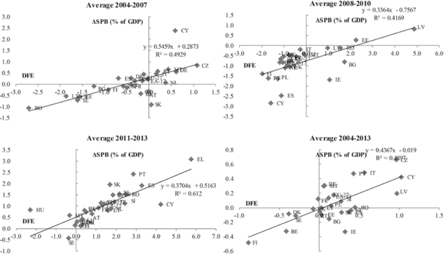
Figure 3. Relationship between the change in the structural primary balance
DQGWKHGLVFUHWLRQDU\¿VFDOHIIRUW
Source: AMECO (Commission Spring 2014 forecast), authors’ calculations.
Overall, the change in the structural primary balance and the discretionary scal effort
display notable correlation. For the entire sample the simple correlation coefcient amounts
to around 0.7. The correlation is stronger before the crisis period than thereafter, especially
between 2011 and 2013. In this period most of the countries adopt consolidation strategies
but the degree of scal tightening shown by the discretionary scal effort often exceeds that
stemming from the change in the structural primary balance (Figure 3). The correlation
between the two indicators also differs between the group of countries that underwent a
more pronounced boom and bust cycle (Cyprus, Ireland, Italy, Latvia, Lithuania, Malta,
Portugal, Romania, Slovenia and Slovakia, Spain and the United Kingdom) and the group
gathering other economies. The correlation between the two indicators is signicantly
stronger in the latter group, than in the former group, suggesting that the information
brought by the discretionary scal effort is more signicant when economies experience
large shocks.
3.3. Discretionary scal effort and cyclical position
Figure 4 shows the evolution of the scal stance as measured by both the discretionary
scal effort and the change in the structural primary balance in relation with the economic
cycle for the euro area and for the EU-27. These charts allows a rough characterisation of
the scal path as either «pro-cyclical» (a positive scal effort in bad times, or a negative

76
effort in good times), «counter-cyclical» (the two opposite situations), or possibly close to
neutral. To do this requires some simplifying assumptions. In particular, we construct a
summary indicator of business conditions combining information from the level and the
change in the output gap
8
.
According to this approach, the scal stance as measured by the discretionary scal ef-
fort may be said to have been close to neutrality over the pre-crisis years of 2004-2007 in the
context of increasingly favourable conditions (in the detail, there was a modicum of initial
countercyclical tightening in 2004 in the euro area, and mild pro-cyclical loosening in the
mid-2000s for the EU-27). This suggests that overall the «good times» were not or not much
taken advantage of for strengthening budgetary positions. By contrast, the change in the
structural primary balance would suggest a countercyclical tightening taking place over the
same period.
With the «Great Recession» of 2008-2009 the scal stance changed gear dramati-
cally. The stimulus packages adopted to counter the effects of the pronounced recession
in 2009 led to a counter-cyclical scal loosening. However, as part of a strategy of
gradual consolidation amplied by the outbreak of the sovereign debt crisis in the euro
area especially affecting several «peripheral» economies, most governments started to
implement signicant consolidation measures as of 2010. While this initially occurred
against the background of a mixed economy, as economies bottomed out of the recession
in 2010-2011, this strategy generally evolved into signicant pro-cyclical tightening in
2012-2013. The overall impression is that scal policies have been conducted in a some-
what stop and go and fashion, without much counter-cyclical action, except in the early
stage of the crisis.

77
The Discretionary Fisical Effort: An assessment of Fiscal Policy and its Output Effect
)LJXUH 7KH¿VFDOVWDQFHDQGWKHF\FOH
Source: AMECO (Commission Spring 2014 forecast), authors’ calculations.
Despite some differences across countries, this picture is broadly observed in most coun-
tries, namely Belgium, the Czech Republic, Spain, France, Italy, Cyprus, the Netherlands,
Portugal, Slovenia, Slovakia, Finland and the United Kingdom. Ireland shows a similar pat-
tern too, although the sharp pro-cyclical tightening took place in 2008, instead of 2009 as
observed in other cases, due to the earlier effects of the banking crisis derived from the
earlier collapse of the housing market. In turn, due to data availability we can only offer this
relationship for Greece for the period 2011-2013, when a pronounced pro-cyclical tightening
derived from the requirements of the macroeconomic adjustment programme is detected
9
.
4. Estimating scal multipliers
This section uses the natural properties of the discretionary scal effort as an indicator
of the scal stance to estimate, based on the panel data analysed in section 3, the short-term
impact on activity of scal policy, as well as its dependence on the composition of scal
shocks and the state of the economy.
4.1. Methodology
The most direct way to empirically evaluate short-term (1-year) scal multipliers is to
estimate the following specication:
y = m DFE + β y + Γ X + c + ε
(2)
it y it i it−1 i it i it
where y
it
is real annual output growth for country i and year t, X
it
is a vector of control fac-
tors, c
i
are country-xed effects, and m stands for the (one-year) output multiplier
10
.
y
78
The above specication is estimated for an unbalanced panel comprising 27 EU Member
States over the period 2004-2013, using the data presented in previous sections.
In multiplier regressions of this kind, a typical problem when relying on the structural
balance as an indicator of scal shocks, is the potential endogeneity to economic develop-
ments. This essentially stems from the large revenues windfalls and shortfalls associated
with good and bad times respectively, which induce a contemporaneous correlation between
changes in the structural balances and output growth that biases the estimated value of the
multiplier. In addition, the potentially pro-cyclical nature of potential growth is another pos-
sible source of endogeneity.
The discretionary scal effort is, by construction, much less exposed than the structural
balance to these endogeneity issues, because it relies on a bottom-up approach on the reve-
nue side, and because it uses a smoother notion of potential growth that is less likely to ex-
hibit pro-cyclicality. However, while that would make it a natural candidate to serve to
identify scal shocks in a multiplier regression, including using a basic OLS framework,
some degree of endogeneity in the discretionary scal effort through its reliance on smoothed
potential growth may remain.
Moreover, another potential source of endogeneity would arise if scal policy measures,
in particular revenue measures, responded contemporaneously to the prevailing economic
conditions (in other words, a systematic scal policy reaction function with contemporane-
ous growth entering as an argument). It is unclear whether such contemporaneous reaction
can be found empirically (see Born and Müller, 2012; Beetsma et al., 2009). However, there
is anecdotal evidence of this in at least occasional episodes, such as large counter-cyclical
response at the 2009 trough (see Section 3.3). In our case, neither the DFE nor its compo-
nents can be taken as exogenous to underlying economic conditions. To test this hypothesis
we run a set of Granger causality tests and in all cases the null hypothesis that GDP growth
does not Granger-cause the scal effort was rejected.
These problems advise against simple OLS estimates and call for a more robust estima-
tion strategy. Accordingly, we estimate alternative versions of equation (2) by GMM by using
the estimator proposed by Arellano and Bover (1995) and further developed by Blundell and
Bond (1998) for dynamic panel datasets, which offers consistent estimates.
11
We use the
typical GMM instruments for this estimator, namely the usual lagged levels and differences
of the dependent and DFE variables, and the levels and rst differences of the exogenous
variables included in the models. The validity of the instruments used is tested with the
Hansen J test.
The US GDP growth rate is included in all specications as a proxy for a wide range of
common economic factors, in particular extra-EU foreign demand. Moreover, we included a
monetary conditions index (mci). This index is obtained as a weighted average of the real
short-term interest rate and the real effective exchange rate relative to their value in a base
period
12
.
79
The Discretionary Fisical Effort: An assessment of Fiscal Policy and its Output Effect
Furthermore, we also controlled for external scal shocks. In this regard, Beetsma et al.
(2008) and In’t Veld (2013) show that spillovers of scal shocks are large, which add to the
direct effects of domestic scal shocks on GDP. These effects are especially relevant when
some degree of coordination of scal policies takes place. Arguably, this has been the case
after the outbreak of the nancial and economic crisis since 2008. At earlier stages sizeable
stimulus packages were adopted by a number of Member States, whereas from 2010 on-
wards most countries engaged in scal consolidations. Accordingly, we included a country-
specic measure of external scal shocks gauged as the weighted average of the discretion-
ary scal efforts of other Member States. The weights used in this case were those of
national GDPs on total EU GDP.
4.2. Results
The scal multipliers obtained in the framework described above are shown in Table 2.
The average rst-year multiplier is estimated at around 0.75 (given lags, the second-year
multiplier is slightly above unity). Such values might be seen as relatively middle-of-the-
road, in comparison with previous empirical studies, although the evidence is quite dispersed
(see for instance Coenen et al., 2012; Barrell et al., 2012; or European Commission, 2012).
Our results are also broadly consistent with model-based simulations of the QUEST model
(see Roeger and In’t Veld, 2010, which also highlights the composition and state-dependen-
cy of the multipliers). Model (2) includes the lagged «discretionary scal effort» and its
components as regressors, but in no case were lagged scal shocks signicant.
The estimated coefcient of US growth is very high, at above one. While such a high
value may seem somewhat surprising, this coefcient is intended to capture not only direct
effects from US growth, but also the broad range of external factors affecting euro area
economies over the sample period, in particular during the crisis years. Finally, the monetary
conditions index is always non-signicant and this is the reason why it is removed from
model (3). Contemporaneous and lagged «external discretionary scal efforts» are included
in all specications, but only the latter turns out to be signicant in all specications, con-
rming the presence of some spill-over effects over the sample period, especially following
the outbreak of the crisis. The signicance of the lagged coefcient indicates that scal spill-
overs take some quarters to develop fully. As expected, the accumulated spill-over effect
captured by these coefcients is of lower magnitude than the direct effect stemming from
domestic scal shocks. In any case, the spill-over coefcients are remarkably high in all
specications, e.g. when compared with the results in In’t Veld (2013). This could be due to
strong spill-over effects in small Member States that that are not assessed in In’t Veld (2013)
in that it only focusses on a selection of countries.
Revenue and expenditure multipliers can be estimated by using as scal shocks the rev-
enue and expenditure sides of the DFE in isolation, i.e. the rst and second term, respec-
tively, of equation (2). Hence, our scal multipliers to revenue shocks are obtained in accord-
ance to a narrative approach. Conversely, by construction, expenditure multipliers gauged

80
with the DFE would be methodologically closer to those obtained under a top-down ap-
proach, albeit with renements as discussed earlier.
Both expenditure and revenue multipliers take the expected sign, although only ex-
penditure multipliers turn out to be signicant at conventional levels. First-year expenditure
multipliers are estimated at between 0.9 and 1.0, whereas revenue multipliers turn out to be
lower, at around 0.35 (with second-year responses always about a third higher).
Table 2
ESTIMATED OUTPUT MULTIPLIERS
dfe
t
dfe
t-1
drm
t
drm
t-1
dfe_g
t
dfe_g
t-1
y
t-1
y
US
t
mci
t
dfe*
t
dfe*
t-1
const
Obs.
Hansen test of overidentifying
restrictions
GMM (1)
-0.76***
(0.23)
0.32***
(0.07)
1.60***
(0.18)
0.02
(0.03)
0.29
(0.43)
-0.87***
(0.27)
-1.54***
(0.47)
219
χ
2
(36) =
24.82
GMM (1)
-0.35
(0.25)
1.02***
(0.32)
0.30***
(0.07)
1.53***
(0.20)
0.02
(0.03)
0.46
(0.43)
-0.95***
(0.29)
-1.48***
(0.51)
219
χ
2
(52) =
24.45
GMM (2)
-0.60**
(0.26)
0.16
(0.13)
0.35***
(0.06)
1.59***
(0.20)
0.01
(0.03)
0.28
(0.51)
-1.08***
(0.37)
-1.62***
(0.31)
213
χ
2
(51) =
25.21
GMM (2)
-0.22
(0.46)
0.08
(0.30)
0.81***
(0.22)
-0.18
(0.20)
0.35***
(0.06)
1.51***
(0.17)
0.01
(0.03)
0.40
(0.37)
-1.20***
(0.38)
-1.55***
(0.33)
213
χ
2
(72) =
22.76
GMM (3)
-0.75***
(0.23)
0.33***
(0.06)
1.59***
(0.15)
0.31
(0.41)
-0.90***
(0.26)
-1.47***
(0.27)
219
χ
2
(37) =
24.76
GMM (3)
-0.35
(0.24)
0.90***
(0.25)
0.33***
(0.05)
1.53***
(0.14)
0.34
(0.35)
-0.95***
(0.28)
-1.41***
(0.25)
219
χ
2
(53) =
23.76
Notes: Robust standard errors in brackets. The symbols ***, ** and * indicate that the coefcient is signicant at the
1%, 5% and 10% signicance levels, respectively.
Variables: dfe: discretionary scal effort; drm: discretionary revenue measures; dfe_g: discretionary effort on the
expenditure side; y: real GDP growth; y
US
: US real GDP growth; mci: the monetary conditions index; dfe*: country-
specic external DFE.
The estimated expenditure multipliers fall comfortably within the range of values ob-
tained in other empirical studies (see Romer and Bernstein, 2009; Christiano, et al., 2011; De

81
The Discretionary Fisical Effort: An assessment of Fiscal Policy and its Output Effect
Castro, 2006; De Castro and Hernández de Cos, 2008; Giordano et al., 2007, among others).
In particular, expenditure multipliers are in line with those in Burriel et al. (2010) for the euro
area as a whole. In turn, although non-signicant, revenue multipliers seem also in accordance
with estimates in Biau and Girard (2005), Giordano et al. (2007), Perotti (2004) or Cloyne
(2011), whereas they are a bit lower than those in Burriel et al. (2010) for the euro area
13
.
Table 3
OUTPUT MULTIPLIERS IN BAD TIMES (∆YGAP<0)
GMM GMM GMM GMM
dfe*
t
-0.27
(0.29)
-0.29
(0.24)
dfe*bad
t
-0.81***
(0.31)
-0.81***
(0.29)
drm
t
0.04
(0.45)
0.07
(0.46)
drm*bad
t
-1.45**
(0.60)
-1.50**
(0.60)
dfe_g
t
0.71**
(0.28)
0.68**
(0.28)
dfe_g*bad
t
0.40
(0.34)
0.35
(0.38)
0.36***
0.37***
0.28*** 0.29***
y
t-1
(0.06)
(0.06)
(0.06) (0.06)
y
US
t
1.70***
(0.16)
1.69***
(0.15)
1.55***
(0.20)
1.53***
(0.18)
mci
t
0.02
(0.03)
0.02
(0.03)
dfe*
t
0.24
(0.42)
0.25
(0.41)
0.42
(0.40)
0.35
(0.41)
dfe*
t-1
-0.73**
(0.32)
-0.78***
(0.29)
-0.63**
(0.30)
-0.63**
(0.29)
const
-1.71***
(0.35)
-1.54***
(0.29)
1.49***
(0.47)
-1.31***
(0.29)
Obs. 219 219 219 219
Hansen test of overidentifying
χ
2
(35) = χ
2
(36) = χ
2
(50) = χ
2
(51) =
restrictions
25.56 26.69 20.52 21.43
Notes: Robust standard errors in brackets. The symbols ***, ** and * indicate that the coefcient is signicant at the
1%, 5% and 10% signicance levels, respectively.
There is a growing acceptance that output multipliers are higher in «bad times» than in
«good times». This can be for a number of reasons (see Auerbach and Gorodnichenko, 2011,
2012; Christiano, et al., 2011; Eggertson and Krugman, 2012; Blanchard and Leigh, 2013).
In particular, scal multipliers are deemed to be higher in an environment of weak activity,
lack of room for supporting monetary policy close to the zero lower bound and tight nancing
constraints for private agents. Conversely, in an economy without slack the effect of

82
expansionary spending policies are thought to be crowded out by lower private consumption
or investment.
To explore this idea, we take two different approaches: rst, we interact the «discretion-
ary scal effort» with a dummy capturing «bad times» that takes ones when the change in
the output gap is negative and zeroes otherwise
14
; second, we split the sample into «good
times» and «bad times» according to the same criterion and estimate separately
15
.
In the former case, Table 3 shows that the interaction between the «discretionary scal
effort» and the dummy variable capturing bad times is signicant in both specications and
contributes to increasing the scal multiplier. This effect stems mainly from the effect on the
revenue multiplier, whereas the interaction coefcient in not signicant in the expenditure case.
Table 4
OUTPUT MULTIPLIERS IN GOOD AND BAD TIMES
∆ygap≥0 ∆ygap<0
-0.71***
(0.27)
-0.63**
dfe
t
(0.31)
-0.59**
(0.28)
-0.70***
(0.23)
drm
t
-0.00
(0.55)
-0.09
(0.20)
-0.56
(0.40)
-0.55
(0.35)
dfe_g
t
0.96***
(0.28)
0.88***
(0.33)
0.91***
(0.35)
0.97***
(0.34)
0.29** 0.21* 0.30*** 0.30** 0.66*** 0.57*** 0.60*** 0.33***
y
t-1
(0.12) (0.11) (0.11) (0.13) (0.11) (0.11) (0.10) (0.05)
1.60***
y
US
t
(0.19)
1.62*** 1.56***
(0.20) (0.19)
1.57***
(0.17)
1.78***
(0.29)
1.74*** 1.82***
(0.25) (0.31)
1.80***
(0.25)
0.05
mci
t
(0.04)
0.04
(0.04)
-0.03
(0.12)
-0.05
(0.06)
0.39
dfe*
t
(0.43)
0.18 0.39
(0.44) (0.44)
0.48
(0.50)
-0.29
(0.51)
-0.21 -0.36
(0.28) (0.47)
-0.26
(0.37)
-0.42
dfe*
t-1
(0.53)
-0.29 -0.41
(0.48) (0.49)
-0.71
(0.68)
-0.60*
(0.36)
-0.67** -0.52*
(0.34) (0.28)
-0.64*
(0.34)
-1.05**
const
(0.51)
-0.96 -0.84*
(0.49) (0.45)
-1.06
(0.54)
-2.59***
(0.51)
-2.37*** -2.68***
(0.32) (0.40)
-2.46***
(0.33)
Obs. 125 125 125 125 94 94 94 94
Hansen test of overidentifying
χ
2
(32) = χ
2
(66) = χ
2
(33) = χ
2
(47) = χ
2
(30) = χ
2
(44) = χ
2
(33) = χ
2
(45) =
restrictions
23.22 24.25 23.88 23.92 24.85 23.02 25.58 22.83
Notes: Robust standard errors in brackets. The symbols ***, ** and * indicate that the coefcient is signicant at
the 1%, 5% and 10% signicance levels, respectively.
Table 4 presents output multipliers for «good» and «bad times» separately. Fiscal mul-
tipliers tend to be lower than average in good times, with revenue multipliers at around 0.1
and expenditure multipliers at 0.9. However, while differences in expenditure multipliers
83
The Discretionary Fisical Effort: An assessment of Fiscal Policy and its Output Effect
are negligible (multipliers are estimated at between 0.9 and 1.0 in both cases), revenue
multipliers in bad times are increased to over 0.5, though remaining non-signicant at con-
ventional levels.
4.3. Caveats
The insights presented in this section are generally not overly surprising, but the esti-
mates have to be taken with care as they are based on a very short time span and accord-
ingly rely on a small number of observations.
Some other caveats should be borne in mind too. In general, the estimated magnitude of
scal multipliers signicantly depends on the composition of the scal shocks. The level of
granularity needed to account for the composition-dependency found in the literature goes
beyond the aggregate categories of expenditure and revenues used here. While in principle it
would be possible to break down further the discretionary scal effort, we do not attempt
such extension in this work because we do not have the necessary breakdown for discretion-
ary revenue measures.
Moreover, the multipliers presented above should be seen as average values over EU coun-
tries. They are calculated over twenty-seven countries enjoying differing characteristics and
expected responses to policy moves. Fiscal multipliers are generally thought to be somewhat
country-dependent and the panel approach can only deliver an average value. In an extension
to the basic specications reported above, we have tried to identify differences in multipliers
stemming from the degree of openness, one of the most-widely acknowledged origins of coun-
try differences (Barrell et al., 2012). Our results are in accordance with the assumption that
overall multipliers tend to decrease with openness, though the coefcients for the expenditure
or revenue components estimated separately are not signicant at conventional levels
16
.
It may also be worth recalling that one-offs and other temporary measures are netted out
to calculate the discretionary scal effort, for which the scal shocks used to estimate the
multipliers are either permanent or relatively long-lasting. As permanent scal shocks are
deemed to entail lower multipliers than transitory ones, the estimates presented here might
be downward biased when compared to other papers.
5. Conclusions
The comparison between the change in the structural primary balance and the discretion-
ary scal effort suggests that the former yields a more optimistic view of the orientation of
scal policy in booms, while it tends to underestimate the scal effort in recessions. Relying
on enacted measures on the revenue side and on medium-term potential growth on the ex-
penditure side, the discretionary scal effort seems to yield a better evaluation of the under-
lying orientation of scal policy when economies are exposed to shocks that are ill-captured
84
by standard estimates of cyclical tax and spending elasticities, large changes in interest pay-
ments, or sharp revisions in potential growth.
The empirical part of this paper conrms that the description of scal policies is to an
important extent inuenced by the choice of approach. In particular, the discretionary scal
effort suggests that, with exceptions, scal policy in the EU has been conducted in a more stop
and go and pro-cyclical fashion over the past ten years than suggested by traditional indica-
tors. In recent years, in a context when most EU countries are tightening scal policy, the
actual consolidation effort appears to be underestimated in many countries when assessed on
the sole basis of the structural balance. Conversely, during the booming years that preceded
the crisis, the structural balance tended to overestimate the progress on scal consolidation.
Using the discretionary scal effort, the average rst-year scal multiplier is estimated
at a below unity on average, with the aggregate expenditure multiplier being signicantly
larger than the aggregate revenue multiplier. We also nd some differentiation between good
and bad times as dened by a positive (respectively negative) change in the output gap, with
average multipliers being lower in the former case. Signicant limitations of our empirical
work, however, relate to the relatively limited time span, the uncertainty in parts of the data
(notably the yields of tax measures in early years of the panel), and the panel approach which
only allows us to estimate an average, non-country dependent multiplier.

85
The Discretionary Fisical Effort: An assessment of Fiscal Policy and its Output Effect
Annex A. Analytical decomposition of the difference between the
change in the structural balance and the discretionary scal effort
17
To recall, the discretionary scal effort is dened as:
N
R
∆E − .
−
)(
pot E
R G
t
t t 1
DFE = DFE +DFE = −
(A.1)
t t t
Y
t
Y
t
with the N
R
budgetary impact of revenue measures in year t, E adjusted general government
t
expenditure adjusted and pot is medium-term nominal potential growth.
The structural balance is the cyclically-adjusted balance corrected for one-offs and other
temporary measures
18
:
R G
r
0
g
0
SB R G − S −1 − S −1 OG=−
( ) ( )
(A.2)
t t t 0 0 t
Y
0
Y
0
where R
t
and G
t
are general government revenues and expenditure respectively, both ad-
justed for one-offs and other temporary measures, BAL = R
t
is the general government
t
– G
t
balance, and OG is the output gap. The parameters ρ
0
r
and ρ
g
are the cyclical revenue and
t 0
expenditure elasticities. Equation (A.2) can also be written: SB = BAL – ε. OG
t
where
t t
r
0
g
0
ε =
(
ρ
0
−1
)
R
−
(
ρ
0
−1
)
G
is the semi-elasticity of the budget balance to the output gap
19
.
Y
0
Y
0
The change in the structural balance (ΔSB) can be decomposed into a contribution from
the revenue side (∆SBR) and a contribution from the expenditure side (∆SBG).
The revenue contribution can be expressed as:
∆
R
R R R
SB =
t t
−1
r
0
t
− −
(
S
0
−1
)
(OG
t
- OG
t−1
)
Y
t
Y
t
−1
Y
0
or equivalently
R
R
t
R
∆
t
−1
(
r
R
SB = − − S −1
)
0
Y
0
(
*
t
yy
t
-)
t
(A.3)
t
Y
t
−1
Y
0
where and denote the actual and potential GDP growth rates, respectively.
And the expenditure contribution is similarly:
G G
G
SB
G
∆ =−
t
−
t
−1
t
+
g
(
S
−
1
)
0
(yy-)
*
(A.4)
Y
0 t t
t
Y
t
−1
Y
0

86
On the revenue side:
The revenue contribution to the difference between and the DFE is the difference be-
R
R
N
t
tween expression (A.3) and
DFE
:
t
Y
t
R R N
R
R
R R
t t
−1
t
r
0
*
(A.5)
(
−
)
(--)∆SB − DFE = − − − S 1 y y
t t 0
t
t
Y Y Y Y
t t
−1
t
0
To give a simpler form to this expression, let’s dene the actual (i.e., observed, by contrast
to the average) semi-elasticity of revenues (after netting out discretionary measures)
S
t
r
as:
r
(
R
t
−
N
R
t
−
R
t−1
)
/ R
t−1
R
t
R
t−1
N
t
R
r
R
t
−1
S
t
=
, or equivalently
− −
=
(
S
t
−1
)
y
Y Y Y Y
(
Y −Y
) /
Y
t t−1 t
t
−1
t t−1 t−1
Plugging this expression into (A.5) and rearranging yields the following decomposition
for the difference between ΔSB and the DFE on the revenue side:
R R R
R
R R r r
0
r *
0
r
t−1 0
∆SB − DFE =
(
S −S
)
y +
(
S −1
)
y +
(
S −1
)
y
−
(A.6)
t t t 0 0 t t t
Y Y
Y
Y
0 0 t−11 0
The three terms in (A.6) have a clear economic meaning:
i. The rst term in the right hand side is an approximate measure of revenue windfalls/
shortfalls, which shows up as the difference between the actual and average elasticities.
Empirically, this is by far the largest contributor to the difference on the revenue side.
ii. The second term reects a possible inertial increase/decrease in the revenue-to-GDP
ratio linked in the event of a non-unitary (average) elasticity of revenues to output. In
general, this is small as most values of
S
0
r
do not much differ from unity.
iii. The last term is a residual term that appears when the actual share of expenditure
departs from the share in the base year. In practice, this is quantitatively small as well.
On the expenditure side:
The expenditure contribution to the difference between and the DFE is:
G G
G G I U
+SB
g G
t
−
t 1
g
+
t
− DFE
−
t
= −
(
S
0
−
1
)
0
−−
(
*
t
yy
t
t
Y
t
-
t
))+
t
−
Y
t
−1
Y
0
Y
t
G
t
−1
−
I
t
−
U
−+
(
1
pot
−1
t
−1
(A.7)
)
Y
t

87
The Discretionary Fisical Effort: An assessment of Fiscal Policy and its Output Effect
Notice that in (A.7) total unemployment expenditure, instead of non-discretionary un-
employment expenditure is deducted. By rearranging terms (A.7) can be written as:
G G I ∆U I U
g G
t
−1
g
0
*
t t
t−1
+
t−1
∆SB − DFE = −y pot
)
+
(
S −1 (yy-)−∆ − − −
(
y pot
)
(A.8)
t t
(
0
)
t t
t
Y Y Y
YY Y
t
−1 0
t
t t−1
Similarly to what we did on the revenue side, the expression can be simplied by introduc-
ing the actual (i.e. observed, by contrast to the average) unemployment expenditure elasticity
(
U
t
−U
t−1
)
/ G
t−1
S
t
g
=
*
y
t
− y
t
g
*
G
Substituting in (A.8) and assuming that the term
S
)
t−1
t
(
y
t
− y
t
is at rst order equiv-
Y
t
alent to
S
g
(
y − y
*
t t t
)
the following expression after some algebraic manipulation is obtained:
∆SB
g
t
− DFE
G
t
=
(
S
g g
G
*
+
*
pot
)
G
−S
)
0
(y -)y
(
y −
t −1
I
−∆
t
0 t t t t
++
Y
0
Y
t−1
Y
t
(A.9)
G G
(
1
g
)
-)
*
+−S (yy
t−1
−
0
I +U
t t t
−
(
y
−
t−1 t−−1
t
pot
)
Y Y
t−1 0
Y
t−1
As in the case of revenues, the different terms in equation (A.9) have a clear economic
interpretation:
i. The rst term on the right hand side reects the «windfalls/shortfalls» in unemploy-
ment expenditure.
ii. The second term stems from the variability of potential growth, and reects the gap
between the usual «annual» potential growth and the smoother notion that we adopt
in the discretionary scal effort.
iii.The third one merely shows the effect of the increase in interest payment expendi-
ture. Such source of difference between both indicators is overcome by the use of the
change in the cyclically adjusted primary balance (∆SPB), instead of ∆SB.
iv. The fourth term shows up as due to the deviation of expenditure ratios with respect
to the xed weights used in the structural balance methodology.
v. Finally, the fth term reects the excess trend projection of interest and unemploy-
ment expenditure with respect to the medium-term potential growth rate.
As can be expected, the last two terms are small in practice when compared to the other
three ones.

88
Annex B. Discretionary revenue measures
Discretionary revenue measures can be dened as changes in policy that have a direct
impact on the revenues of general government. In general, a discretionary revenue measure
implies a legislative or administrative act, though there are some borderline cases.
20
Eco-
nomically, changes in public revenues can be split in two parts, one reecting the impact of
new discretionary measures, the other the «spontaneous» developments in the economy.
Such a decomposition is typically used when forecasting or analysing revenue developments.
Importantly, what should be accounted as the effect of a discretionary measure in a given
year is its «additional» impact in that year. A measure that is phased in (or phased out) over
several years therefore has successive incremental impacts over these years.
Figure B.1. Discretionary revenue measures, EU countries, 2004-2013
Source: AMECO, Output Gap Working Group, authors’ calculations.
Within the context of EU scal surveillance, growing attention has been paid in recent
years to the evaluation of discretionary revenue measures. In the framework of the Output
Gap Working Group of the Economic Policy Committee, Member States are asked to annu-
ally report data on discretionary measures on the basis of a common questionnaire (Princen
and Mourre, 2014). Recent efforts have focused on reaching a common denition of discre-
tionary measures, providing guidance on the reporting of complex measures, ensuring a
89
The Discretionary Fisical Effort: An assessment of Fiscal Policy and its Output Effect
comprehensive reporting (encompassing the whole general government, including in par-
ticular local governments and social security contributions), and encouraging Member
States to report data back from the early 2000s. The increased scrutiny of discretionary
measures for the purposes of scal surveillance, by the European Commission but also
potentially by national scal councils, acts as an incentive for Member States to improve
the quality and transparency of their reporting. This being said, there also remains room for
further progress in ensuring the robustness, full comparability, and public availability of the
estimates.
The available data point to a great variety of experiences with discretionary revenue
measures (Figure B.1). In a given year, both tax hikes and tax cuts are observed across the
group of EMU countries. However, there is a dominance of tax cuts in the pre-crisis period,
and also in the early phase of the crisis as governments embarked on stimulus packages, fol-
lowed by a large prevalence of tax increases in the ensuing consolidation period. On average
over the past decade, cuts and hikes tend to broadly offset each other’s, at least when taking
the EMU countries as a whole, with the panel average of measures at a mere 0.08% of GDP.
However, for individual years and countries, the size of revenue measures can be quite large,
sometimes exceeding 1% or even 2% of GDP in absolute value.
Notes
1.
Or the change in the structural primary balance. In the usual EU terminology, the structural balance is dened as
the cyclically-adjusted balance net of one off and other temporary measures. For a presentation and discussion
of the EU methodology, see Larch and Turrini (2009) and Mourre et al. (2013).
2.
This part of the paper expands on work presented in European Commission (2013).
3.
The aggregate elasticity of tax revenues to output is typically taken to be close to unity, although elasticities
of specic tax categories, such as personal income or corporate taxes, may differ signicantly. See Mourre et
al. (2014).
4.
The variable pot as set above is multiplied by GDP deator ination before entering equation (1), so that
the nominal growth of the expenditure aggregate E is benchmarked against a notion of «nominal» potential
growth.
5.
There are four differences between the discretionary scal effort and a literal reformulation of the ex-
penditure benchmark as an indicator of the scal stance: rst, the expenditure benchmark smoothens
public investment over four years; second the expenditure benchmark nets out government expenditure
programmes fully matched by revenues from EU funds; third, to relate nominal expenditure and real
potential growth, the expenditure benchmark employs the average of the GDP deator ination forecasts
for year t made by the Commission in spring and autumn of year t-1, while the discretionary scal effort
uses the actual GDP deator ination; fourth, the discretionary scal effort corrects for one-offs and other
temporary measures in the same way as the structural balance. The choices made for the expenditure
benchmark have a history of their own. However, from the point of view of building an indicator of the
underlying scal stance as well as for reasons of simplicity, the choices made for the discretionary scal
effort seem preferable.
6.
The term revenue windfalls/shortfalls used here is broader than in other papers in the literature. More precisely,
the difference between the two indicators stemming from the differences between observed and standard ag-
gregate elasticities used for cyclical adjustment purposes can be due to the decoupling of tax base proxies from
90
GDP, composition effects affecting the different tax categories and the truly unexplained changes, the genuine
«revenue windfalls/shortfalls» (see Morris et al., 2009). However, we use a broader denition, which has the
advantage of enabling a natural comparison of the DFE properties with the top-down approach of the structural
balance that is commonly used in EU scal surveillance. In our approach, it is acknowledged that «windfalls»
(or shortfalls) encompass a mix of composition effects, idiosyncratic responses of specic taxes, and a great
diversity of «technical factors.»
7.
The change in the structural balance is not presented to ensure a more direct comparison in that the change
in interest payments is one of the main explanatory factors behind the difference between the two indicators.
Annual potential output and smoothed potential output are calculated based on ex-post data as opposed to real
time data. This applies to both indicators of the scal stance.
8.
There is no universally agreed metric of cyclical conditions. While the output gap is the natural starting point
(see, for instance, Galí and Perotti, 2003, or Alesina et al., 2008), it may be an insufcient or even possibly
misleading gauge at times. The literature suggests that the change in the output gap may offer a complementary
and more robust signal (see European Commission, 2006, Part IV, or OECD, 2003). Accordingly, we construct
a composite indicator giving equal weights to the output gap and the change thereof. Specically, the difference
between the output gap and its centred average is divided by its standard deviation, which generally falls (but
not always) between [-2; +2]. We proceed similarly with the change in the output gap. The composite indica-
tor is computed as the simple average of the normalised output gap level and the normalised change in the
output gap, which generally falls within the interval [-2; +2], although it can fall outside this band in unusual
circumstances.
9.
This relationship between the economic cycle and the scal stance by country as measured by the discretionary
scal effort is available upon request.
10.
In order to strictly preserv e the denition of the multiplier as the euro change in output per euro of ex
ante relaxation of the budget balance, the DFE is multiplied by a factor Y
t
/Y
t-1
when entering the above
regression.
11.
These models were estimated in Stata with the command xtabond2 de
veloped in Roodman (2009). This esti-
mator is especially recommended for panels, like the one we are dealing with, characterised by a signicant
cross-country dimension and few time periods.
12.
The weights reect each v
ariable’s relative impact on GDP after two years and are derived from simulations in
the OECD’s Interlink model.
13.
Baum and K
oester (2011) and Bénassy-Quéré and Cimadomo (2006) obtain higher revenue multipliers, in the
latter case even exceeding 1.
14.
Another possibility here w
ould have been to dene the cycle in terms of the medium-term potential growth
rate, in line with the benchmark used for assessing the scal effort on the expenditure side. However, the ap-
proach we follow here is more aligned with the usual denition of cycle used by most international institutions,
academics and analysts.
15.
Admittedly this is a rather crude approach to distinguish between good and bad times, b
ut we opted for this op-
tion because our sample is too short. In general, a more appropriate way to tackle the issue of state-dependent
scal multipliers would be to estimate Markov-switching models with transition probabilities, See, for instance,
Auerbach and Gorodnichencko (2011), Auerbach and Gorodnichencko (2012), Baum and Koester (2011) or
Hernández de Cos and Moral Benito (2015), among others.
16.
These results are a
vailable upon request.
17.
See also European Commission (2013).
18.
Throughout the calculations, we assume that the output gap is sufciently small that terms of second order can
be neglected as compared to rst-order terms. To simplify expressions, we do not explicitly write the adjust-
ment for one offs.
19.
In the current EU methodology
, the weights used to calculate the cyclical budgetary semi-elasticity are time
invariant and obtained as the 10-average average of tax-revenues and expenditure-to-GDP ratios between 2002
and 2011 (denoted by the subscript 0). See Mourre et al. (2013).
20.
F
or example, if regular practice, the annual indexation of tax brackets to ination may not count as a new meas-
ure from an economic viewpoint, although it may have to be implemented through a legislative or administrative
act. Conversely, the (irregular) non indexation would be counted as a discretionary measure.
91
The Discretionary Fisical Effort: An assessment of Fiscal Policy and its Output Effect
References
Alesina, A. and Perotti, R. (1995), «Fiscal expansions and scal adjustments in OECD countries,
NBER Working Paper», No W5214.
Alesina, A., Campante, F. R. and Tabellini, G. (2008), «Why is scal policy often procyclical?», Jour-
nal of the European Economic Association, 6, pp. 1006–1036.
Arellano, M. and Bover, O. (1995), «Another look at the instrumental variable estimation of error-
components models», Journal of Econometrics 68: 29-51.
Ardagna, S. (2004), «Fiscal stabilisations: when do they work and why?», European Economic Review,
Vol. 48, No 5, pp.1047–1074.
Auerbach A. J. and Gorodnichenko, Y. (2011), «Fiscal Multipliers in Recession and Expansion»,
NBER Working Papers 17447.
Auerbach A. J. and Gorodnichenko, Y. (2012), «Measuring the output responses to scal policy»,
American Economic Journal: Economic Policy, 4, 127.
Barrell R., Holland, D. and Hurst, I. (2012), «Fiscal consolidation: Part 2. Fiscal multipliers and scal
consolidations», OECD Economics Department Working Papers, N°933.
Baum, A. and Koester, G. B. (2011), «The impact of scal policy on economic activity over the busi-
ness cycle – evidence from a threshold VAR analysis», Deutsche Bundesbank. Discussion Paper -
Economic Studies No 3/2011.
Beetsma, R. and Giuliodori, M. (2008), «On the relationship between scal plans in the European
Union: An empirical analysis based on real-time data», Journal of Comparative Economics, 36.
Beetsma, R., Giuliodori, M. and Klaassen, F. (2008), «The Effects of Public Spending Shocks on Trade
Balances and Budget Decits in the European Union». Journal of the European Economic Associa-
tion, 6(2-3), 414-423.
Beetsma, R., Giuliodori, M. and Klaassen, F. (2009), «Temporal aggregation and SVAR identication
with an application to scal policy», Economics Letters, 105, pp. 253-255.
Bénassy-Quéré, A. and Cimadomo, J. (2006), «Changing patterns of domestic and cross-border scal
policy multipliers in Europe and the US», CEPII Working Paper 2006-24.
Biau, O. and Girard, E. (2005), «Politique budgétaire et dynamique économique en France: l’approche
VAR structurel», Économie et Prévision 169–171, 1–24.
Blanchard, O. (1990), «Suggestions for a new set of scal indicators», OECD Economics Department,
Working Paper, No. 79.
Blanchard O. and Leigh, D. (2013), «Growth forecast errors and scal multipliers», American Econo-
mic Review, 103(3): 117-20.
Blundell, R., and Bond, S. (1998), «Initial conditions and moment restrictions in dynamic panel data
models», Journal of Econometrics 87: 115-43.
Born, B. and Müller, G. J. (2012), «Government spending in quarterly and annual time series», Journal
of Money, Credit and Banking, 44 (2-3), pp. 507-517.
92
Burriel, P., de Castro, F., Garrote, D., Gordo, E., Paredes, J. and Pérez, J. J. (2010), «Fiscal policy
shocks in the euro area and the US: an empirical assessment», Fiscal Studies 31(2), 251–285.
Christiano, L., Eichenbaum, M. and Rebelo, S. (2011), «When is the Government Spending Multiplier
Large?», Journal of Political Economy 119(1), 78-121.
Cloyne, J. (2011), «What are the Effects of Tax Changes in the United Kingdom? New Evidence from
a Narrative Evaluation», CESIFO Working Paper No. 3433.
Coenen G., Erceg, C., Freedman, C., Furceri, D., Kumhof, M., Lalonde, R., Laxton, D., Lindé, J.,
Mourougane, A., Muir, D., Mursula, S., de Resend, C., Roberts, J., Roeger, W., Snudden, S., Tra-
bandt, M. and int Veld, J. (2012), «Effects of scal stimulus in structural models», American Econo-
mic Review, Macroeconomics, 4/1: 22-68.
D’Auria, F. Denis, C., Havik, K., Mc Morrow, K., Planas, C., Raciborski, R., Röger, W. and Rossi, A.
(2010), «The production function methodology for calculating potential growth rates and output
gaps», European Economy, Economic Papers, 420.
De Castro, F. (2006), «The macroeconomic effects of scal policy in Spain», Applied Economics, 38,
913-924.
De Castro, F and Hernández de Cos, P. (2008), «The economic effects of scal policy: the case of
Spain», Journal of Macroeconomics, 30, 1005-1028.
Devries P., Guajardo J., Leigh D. and Pescatori A. (2011), «A New Action-based Dataset of Fiscal
Consolidation», IMF Working Paper No. 11/128
Eggertson G. and Krugman, P. (2012), «Debt, deleveraging and the liquidity trap», Quarterly Journal
of Economics, pp.1469-1513.
Eschenbach F. and Schuknecht, L. (2002), «Fiscal balances and asset prices», ECB Working Paper No.
141
European Commission (2006), Public Finances in EMU — 2006, European Economy, N°3/2006.
European Commission (2010), Report on Public Finances in EMU — 2010, European Economy,
N°3/2009.
European Commission (2012), Report on Public Finances in EMU, European Economy, N°4/2012.
European Commission (2013), Report on Public Finances in EMU, European Economy, N°4/2013.
Favero, C. A. and Giavazzi, F. (2010), «Reconciling VAR-based and Narrative Measures of the Tax-
Multiplier», CEPR Discussion Papers No 7769.
Galí, J. and Perotti, R. (2003), «Fiscal policy and monetary integration in Europe», Economic Policy,
18, pp. 533–572.
Giordano, R., Momigliano, S., Neri, S. and Perotti, R. (2007), «The effects of scal policy in Italy:
Evidence from a VAR model», European Journal of Political Economy, 23, pp. 707–733.
Guajardo, J., Leigh, D. and Pescatori, A. (2011), «Expansionary Austerity: New International Eviden-
ce», IMF Working Paper No. 11/158
Hernández de Cos, P. and Moral Benito, E. (2015), «Fiscal multipliers in turbulent times: the case of
Spain», Empirical Economics, forthcoming. DOI 10.1007/s00181-015-0969-0.
93
The Discretionary Fisical Effort: An assessment of Fiscal Policy and its Output Effect
Hers J. and Suyker, W. (2014), «Structural budget balance: A love at rst sight turned sour», CPB
Policy Brief, N°2014-07.
In’t Veld, J. (2013), «Fiscal consolidations and spillovers in the Euro area periphery and core», Euro-
pean Economy - Economic Papers 506, Directorate General Economic and Monetary Affairs (DG
ECFIN), European Commission.
International Monetary Fund (2004), World Economic Outlook, September 2004.
International Monetary Fund, (2010), Chapter 3 World Economic Outlook, October 2010.
Kumar, M., Leigh, D. and Plekhanov, A. (2007), «Fiscal Adjustments: Determinants and Macroecono-
mic Consequences», IMF Working Paper No. 07/178.
Larch, M. and Turrini, A. (2009), «The cyclically adjusted budget balance in EU scal policy making:
A love at rst sight turned into a mature relationship», European Economy, Economic Papers
No.374.
Lendvai J., Moulin, L. and Turrini, A. (2011), «From CAB to CAAB? Correcting Indicators of Struc-
tural Fiscal Positions for Current Account Imbalances», European Economy, Economic Papers No.
442.
Morris, R., Rodrigues Braz, C., de Castro, F., Jonk, S., Kremer, J., Linehan, S., Marino, M. R., Schalck,C.
and Tkacevs, O. (2009), «Explaining government revenue windfalls and shortfalls: an analysis of the
revenue data for selected EU countries», ECB Working Paper Series No. 1114, November.
Mourre, G., Isbasoiu, G. M., Paternoster, D. and Salto, M. (2013), «The cyclically adjusted budget
balance used in the EU scal framework: an update», European Economy, Economic Papers, 478.
Mourre G., Astarita C. and Princen, S. (2014), «Adjusting the budget balance for the business cycle:
the EU methodology», European Economy, Economic Papers, 536.
OECD (2003), «Fiscal stance over the cycle: the role of debt, institutions and budget constraints».
Economic Outlook 74.
Perotti, R. (2004), «Estimating the effects of scal policy in OECD countries», Proceedings, Federal
Reserve Bank of San Francisco.
Princen S., Mourre, G., Paternoster, D. and Isbasoiu, G. M. (2013), «Discretionary tax measures: pat-
tern and impact on tax elasticities», European Economy, Economic papers, N°499, May.
Princen, S. and Mourre, G. (2014), «Short-term developments of revenue elasticities: insights from an
EU country panel, European Economy, Economic Papers, forthcoming.
Ramey V. A. (2011), «Identifying Government Spending Shocks: It’s all in the Timing», The Quarterly
Journal of Economics, Vol. 126(1), pp. 1-50.
Roeger W. and in’t Veld, J. (2010), «Fiscal stimulus and exit strategies in the EU: a model-based analy-
sis», European Economy, Economic Papers, N°426.
Romer, C. and Bernstein, J. (2009), «The Job Impact of the American Recovery and Reinvestment
Plan», http://otrans.3cdn.net/45593e8ecbd339d074_l3m6bt1te.pdf.
Romer, C. and Romer, D. H. (2010), «The Macroeconomic Effects of Tax Changes: Estimates Based
on a New Measure of Fiscal Shocks», American Economic Review, 100, 763-801.
94
Roodman, D. (2009), «How to do xtabond2: An introduction to difference and system GMM in Stata».
Stata Journal 9(1): 86-136.
Turrini A. (2008), «Fiscal policy and the cycle in the Euro Area: The role of government revenue and
expenditure», European Economy, Economic Papers No 323.
Resumen
Este artículo presenta un indicador del tono de la política scal que combina elementos del enfoque
narrativo por el lado de los ingresos, con una versión más renada del enfoque tradicional basado en
el saldo estructural por el lado del gasto. Con estas características, dicho indicador ofrece una imagen
de la política scal que mitiga los problemas de endogeneidad que afectan al cálculo del saldo scal
estructural, a la vez que eluden los problemas de indeterminación que aquejan al enfoque narrativo.
Este indicador se utiliza para añadir evidencia adicional sobre las políticas scales en la UE y para
estimar sus efectos a corto sobre el output en promedio. Nuestros resultados muestran que, salvo ex-
cepciones, la política scal durante la pasada década ha sido más procíclica de lo que sugieren los in-
dicadores tradicionales. El multiplicador scal, en promedio, se estima alrededor de 0.75, con multi-
plicadores mayores (menores) asociados a perturbaciones de gasto (ingresos) y en momentos de
contracción (expansión) de la brecha de producción (output gap).
Palabras clave: Tono de la Política Fiscal; Esfuerzo Fiscal Discrecional; Consolidación Fiscal; Multi-
plicadores Fiscales.
Clasicación JEL: E62, H60.
