
1
Jacqueline Ross,
jacqui.ross@auckland.ac.nz
MICROSCOPY NEW ZEALAND INC. CONFERENCE WORKSHOP 2017
Introduction to Fiji 31 January 2017
Table of Contents
OVERVIEW .................................................................................................................................................. 2
DOWNLOADS .............................................................................................................................................. 2
PLUGINS ...................................................................................................................................................... 2
MACROS ...................................................................................................................................................... 3
MEMORY ..................................................................................................................................................... 3
OPENING FILES .......................................................................................................................................... 4
STATUS BAR ............................................................................................................................................... 5
IMAGE PROPERTIES .................................................................................................................................. 5
LOOK UP TABLES (LUT)........................................................................................................................... 6
SPATIAL CALIBRATION ........................................................................................................................... 7
TOOLS ........................................................................................................................................................ 11
SELECTION TOOLS - EDITING, CROPPING AND CREATING ROIS ............................................... 12
OTHER TOOLS .......................................................................................................................................... 13
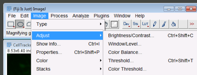
EDIT ............................................................................................................................................................ 16
RESIZING IMAGES ................................................................................................................................... 16
ENHANCING IMAGES ............................................................................................................................. 18
THRESHOLD METHODS ......................................................................................................................... 22
SHADING CORRECTION TOOLS ........................................................................................................... 30
FILTERS...................................................................................................................................................... 32
MORPHOLOGICAL OPERATIONS – BINARY IMAGES ..................................................................... 33
ANALYZE MENU ...................................................................................................................................... 34
IMAGE – STACKS MENU ........................................................................................................................ 35
MOVIES ...................................................................................................................................................... 35

2
OVERVIEW
ImageJ is a public domain image processing program. It was written by Wayne Rasband at the Research
Services Branch (RSB) of the National Institute of Mental Health (NIMH) which is part of the National
Institutes of Health in Maryland, USA. ImageJ is based on Java/javascript (Sun Microsystems) and will run
on any platform. ImageJ has become a standard tool in many laboratories around the world because it is
free, open source, and very well supported. The website address is: http://imagej.nih.gov/ij/
There is a mailing list that you can subscribe to at: http://imagej.nih.gov/ij/list.html
. I recommend this if you
are using the program a lot and want to ask/answer questions but otherwise it’s not necessary since you
can still search the archives without being a subscriber.
There is a very good User Guide to ImageJ available here: http://imagej.nih.gov/ij/docs/index.html
as well
as other information. There is also a Documentation WIKI at: https://imagej.net/Welcome and
http://imagejdocu.tudor.lu/
Fiji is simply a version of ImageJ with a specific compilation of useful Plugins included focused on
microscopy applications. The name of the program is an acronym, which stands for “Fiji Is Just ImageJ”.
Fiji also has a website
dedicated to supporting this particular version of ImageJ with some good tutorials
and documentation.
DOWNLOADS
–available here
There are different versions for each platform or you can use a platform independent version. You do need
Java 6 installed. You can specify which plugins you want to keep updated. You can update manually by
going to Help – Update Fiji. If you are running Windows, it’s recommended that you don’t install the
program in your Program Files folder. The Mac version has a few more options and Help buttons available
in some of the menu items. It also has a Help Search item which isn’t yet available for PC but overall the
versions are very similar.
PLUGINS
Plugins are additional software modules or code, which provide the ability to perform specific tasks.
There is a list of available plugins here: http://imagej.nih.gov/ij/plugins/index.html
. These plugins can be
downloaded and installed in your version of Fiji. In this way, the program can be modified to meet your
particular requirements. To install Plugins/Macros, you can drag and drop onto the Fiji icon. Otherwise,
copy them into the correct folder. To find the folders on the Mac, click on the Fiji icon and RHS mouse click
and go to Show Package Contents. Some plugins have platform-specific versions, others are platform-
independent.

3
You can choose to keep up to date with new versions of any plugins by enabling update sites for those you
use regularly (Help – Update – Manage Updates): more details: http://imagej.net/List_of_update_sites
MACROS
In addition to Plugins, it is also possible to write Macros using several macro languages, e.g. standard
ImageJ1, Javascript, Python, etc. A Macro allows you to string a series of commands together to perform
operations that you may want to do repeatedly. These can also be converted to Plugins by adding an
underscore to the name and putting the file in the Plugins folder. There is a Macro Recorder built into Fiji
that allows you to record each step in a process and then create the Macro. There is also a built-in batch
processing function that can be used to apply processes such as file conversions to entire folders of images
(Process – Batch) storing the results in an Output folder. It can also be used to apply Macros.
Process – Batch –Macro
There are some commonly used built-in options in the drop-down list or you can insert your own!
To insert your own macro, first record all of the steps you need using the Macro Recorder. Create the
macro. Then copy all of the text from the macro into the Batch Processing window, select an Input and
Output folder and click Process to run.
MEMORY
You can change the memory allocation (RAM) if necessary by going to Edit-Options-Memory. Make sure
that you don’t exceed the capability of your computer. You shouldn’t go beyond 75% of your RAM capacity.
If you are opening very large files or stacks, you can use the Virtual Stack option on opening, which only

4
displays the data you are looking at, leaving the rest on the hard drive. Some operations don’t work on
Virtual Stacks and the program can run a bit slower.
OPENING FILES
File-Open: opens TIFF (uncompressed), GIF, JPEG, DICOM, BMP, STK, video and FITS images. It also
opens lookup tables (LUT), text files, regions of interest (ROIs), etc.
File/Import: provides access to Plugins for reading RAW files, images in ASCII format, and for loading
images over the network using a URL. To import a raw (one byte or 8 bits per pixel) file, you must know the
image size (eg. 480x640 pixels) and the offset to the image data.
Files can be opened in groups by selecting them and dragging and dropping them on the ImageJ icon or
onto the toolbar. You can also open files from a series (x-y, lambda, z) by using File-Import-Image
Sequence. The files should be named in numerical order. Fiji will then create a stack for you of the data.
Bioformats plugin – LOCI – part of the Open Microscopy Environment (OME) project – built-in
• Enables you to open files from many different sources and formats. Can also export into some formats.
• Images bring in information such as channel information and calibration.
• “Converts proprietary microscopy data into an open standard called the OME data model
”
Website http://downloads.openmicroscopy.org/bio-formats/5.0.6/
File/Revert: allows you to revert to the last saved version of the image.
File Save: files can be saved in TIFF, GIF, JPEG, AVI, etc., tab-delimited text, and raw formats.

5
STATUS BAR
Gives information such as memory usage:
The position of the cursor (XY pixel coordinates) and Gray or R,G,B, pixel values can also be displayed.
Pixels and Grayscale: Digital images are displayed as "pixels" (short for picture elements). Each pixel is a
spot with a given intensity or greyscale value which is an integer, e.g. in the range 0 (black) to 255 (white) if
it is 8-bit, 0-4095 (12-bit), etc.
IMAGE PROPERTIES
Important information about the image such as resolution, bit depth, type and size is shown in the image
header. Note that the percentage of the image that is currently being displayed is also shown.
Resolution: given in pixels and in microns (or other units) if the image has been calibrated or has been
imported using the Bioformats plugin.
Bit depth: Generally 8, 12 or 16-bits per pixel. 8-bit = 2
8
= 256 gray values; 12-bit = 2
12
= 4096 gray values;
16-bit = 2
16
= 63,536 gray values. Note that these bit depths utilize unsigned integers, positive numbers
only.
Image-Type: allows you to change the image mode. Some operations are designed to work with 8-bit
grayscale or 8-bit colour only. If you want to analyse an RGB image, you may need to change it to 8-bit
colour or grayscale. RGB stands for Red, Green and Blue - each of these intensities can be an integer
between 0 and 255 if the image is 24-bit colour, i.e. 8 bits per channel x 3. Note that 32-bit is used to
approximate “real” numbers as floating point values, i.e. allows decimal points for the pixel values. This type
is used when necessary for some of the more complex mathematical operations.

6
Image-Show Info: displays a list of known information about the image.
Image-Properties: allows you to edit the information about the image, e.g. enter calibration data, etc.
Image – Color: allows you to merge images, change colours, etc. There are also some additional colour
conversions available under this menu.
LOOK UP TABLES (LUT)
Images are displayed using a Look up Table. This assigns a color to be used for each of 256 possible
displayed pixel values (8-bit images). These LUTs are used mainly for fluorescence images but are also
used in other modalities such as medical imaging.
Image – Color -Show LUT: displays the current lookup table of the active image.
Image-Lookup Tables: allows selection of a range of color palettes. There is also a LUT icon on the RHS
of the toolbar that allows direct selection of installed LUTs.
Image – Color – Display LUTS: shows all of the currently installed LUTs.
Image – Color – Edit LUT: allows you to create your own LUT or edit a built-in LUT so that it works better
for your images. You can also open an image with a LUT that you like and save the LUT for use with
another image.
Image – Lookup Tables - Invert LUT: inverts the pixel values.
LUTs are also useful for checking whether you have even or uneven illumination or to assess changes
made when processing images.

7
SPATIAL CALIBRATION
Analyze/Set Scale allows you to calibrate the image so that your results are in units such as microns rather
than pixels. This is very important and should be the first step in your analysis.
If you have a calibration bar on an image, you can use the line tool to draw along it and then go to Analyze
– Set Scale and type in the micron value. Or you can take an image of a micrometer slide with the same
objective lens and magnification and use that to calibrate your images.
Calibrating your images using a micrometer slide image or scale bar
1. When you open your image for the first time, the default calibration may be displayed in inches.
2. Select the Line Tool as shown below (see yellow arrow):
3. Draw a straight line between two of the graduation lines. In this case, the large ones are 500
microns, the intermediate ones are 100 microns and the smallest ones are 20 microns.
4. Draw from the outside of one line to the inside of the next as shown below. Hold the SHIFT key
down to keep the line straight. You should draw the longest line that you can since this will be more
accurate. The line below is 600 microns in length.
8

9
6. Now go to Analyze – Set Scale.
7. A window like the one below will appear;
8. Note the Distance in pixels is highlighted. This is the measurement in pixels of the line that you
have just drawn. The next thing to do is to input the Known distance. In this case, it is 600 microns.
The Unit of length should be entered in microns using the letters um. The Pixel Aspect Ratio
should be 1.0 (X to Y). If you select Global, then all open images will be calibrated the same. If you
open a new image, the program will ask you if you want to use or disable the Global calibration. The
Scale is now shown in pixels/um.

10
9. Click OK. You can see that the calibration is now shown in microns (see yellow arrow below).
Therefore, all measurements will be in microns, microns squared, etc. If you save the image as a
TIFF after calibrating, then the calibration will also be saved.
Scale bars
1. Go to Analyze-Tools-Scale Bar.
2. Choose the size, position, colour, etc. of the scale bar you want.
3. Choose the location using the drop-down box.
4. You can choose to hide the text if you just want a bar.
5. If you want to draw the size of the bar you want or specify a different location on the image to the
options listed, use the line tool to draw a selection first. Choose At Selection for the location. The
bar will be drawn at that location and will be the same length as the selection.
Microscope measurement tools plugin
Author – Demis D. John
Plugin and documentation available here:
http://imagej.net/Microscope_Measurement_Tools
This plugin allows you to store calibration data for different objective lenses for quick and easy calibration of
images. Once the plugin is installed, it will appear at the bottom of the Analyze menu.

11
TOOLS
There are a number of drawing tools on the LHS of the toolbar. Red triangles (as indicated by the arrows
below) indicate more tools/options which are available either by right hand mouse click (Tools) or left/right
hand mouse click (Macro toolsets - Dev/Stk/LUT options). Some tools have options available which are
revealed by double-clicking on the icon, e.g. Line Tool – width, Text Tool (font options).
Stk = shortcut to Stacks menu
Macro toolsets

12
On the RHS, where the >> is located, there are a number of other Tool Sets available which can be
selected. These install macros which change the tool sets visible on the RHS of the toolbar.
SELECTION TOOLS - EDITING, CROPPING AND CREATING ROIS
Most commands in Fiji will work on a region of the image which you need to select or segment in some
way. The default is that the entire image will be analysed. You can also select the whole image by going to
Edit-Selection-Select All.
13
You can define a specific region of interest (ROI) within the image, using any one of the region selection
tools in the Tool Bar (rectangular, oval, polygonal and freehand). To remove a selection, just click the
mouse outside the ROI.
• Rectangle: when using the Rectangle Tool, you can resize by dragging the corners. Hold down the
SHIFT key to constrain the selection to be square. To move the selection, put the cursor inside the
ROI.
• Oval: similar control to the Rectangle Tool, hold down the SHIFT key to get a perfect circle.
• Selection Brush – located under the Oval Tool. Allows you to modify an existing selection.
• Polygon: when using the Polygon Tool, use the left hand mouse click for each vertex, then right
click to close the selection.
• Freehand: when using the Freehand Tool, the gap will be closed automatically with a straight line
as soon as you release the left hand mouse.
Edit – Selection - Specify allows you to specify the size, shape and location of the ROI.
All Selections: use the arrow keys to “nudge” selections one pixel at a time. As a selection is created or
resized, its location, width and height are displayed in the status bar. Selections can be copied, pasted,
cropped, analyzed, etc. using other menu commands. They can also be created from thresholded (red
overlay) or binary images by going to Edit – Selection – Create Selection.
You can create a selection on one image and then transfer it to another image by going to Edit – Selection
– Restore Selection. Create an inverse of any selection by going to Edit – Selection – Make Inverse. To
deactivate a selection, choose the Rectangle Tool and click outside the selection.
Saving Selections: if you save an image with selections on it (but not drawn into the image), then the ROIs
will be there when you open the image again and they remain as Overlays which can be moved/altered.
They can also be transferred to the ROI Manager.
ROI Manager: allows you to store, move, transfer, save and measure ROIs; open it by going to Analyze-
Tools-ROI Manager. Used extensively during analysis.
OTHER TOOLS
Line: Allows you to draw straight, segmented or freehand lines. Double-click on the tool to change the line
width. Go to Edit-Draw to make the line permanent or Ctr-D. The line tool can also be used to plot intensity
across an image – Analyze – Plot Profile.

14
Arrow: You can create arrows by using the Arrow Tool (available when you select the Drawing Tools
under the double-arrow at the end of the tool bar. Double-click on it to change the line width.
Grid: You can apply different types of “grids” to your image by downloading the appropriate plugin
(http://rsb.info.nih.gov/ij/plugins/grid.html
) and installing it. The standard grid plugin allows you to specify
the size of the grid and it can be shown as lines, crosses or points. You can also use a random offset.
Wand: Region-growing tool; allows you to trace the outline of an object or create a selection based on
similar pixel values to the initial sampled value (or “seed”). It also works with a set threshold (Image –
Adjust - Threshold) or a binary image (black/white). You can select multiple objects by holding the SHIFT
key down as you go. Double-click on the tool to see the available options;

15
The Tolerance defines the range of values that will be selected (initial_value-tolerance to
initial value+tolerance), therefore the higher the tolerance, the wider the range of values included.
4-connected only expands selection to neighbouring pixels on each side of the initial sample (“seed”) pixel.
8-connected expands selection to pixels on each side and those diagonally connected to the initial sample
pixel. Selections can be added to the ROI Manager. If you are working on a grayscale image, the option
Enable Thresholding is available;
There is a more sophisticated tool called the Versatile Wand, which provides additional options. It can be
downloaded
and installed in the Plugins folder (included in the workshop version). There is also a Cell
Magic Wand (also included in the workshop version) designed to draw ROIs around individual cells and
add the selection into the ROI Manager – available
here. There is a video showing how to use it and some
good suggestions by the author – Theo Walker. It also works on stacks.
Text: Double-click on the tool to change the options. If the image is grayscale, then text can only be black
or white. If you want coloured text, you need to change the image type to RGB. The colour of the text will be
whatever has been selected as Foreground colour. This can be specified by using the Eyedropper Tool.
You can move the text selection to where you want the text to appear and then go to Edit-Draw (Ctrl-D) to
burn it into the image. Otherwise, it will remain as a selection that can be saved with the image as an
overlay.
16
Eyedropper: Allows you to choose the Background and Foreground colours by double-clicking on the
eyedropper and choosing colours from the Colour Picker. Click on the tiny arrow to swap the Foreground
and Background colours. The colour of the Eyedropper Tool then shows the Foreground colour while
the box around it shows the Background colour. You can also sample colours from an image or select a
colour from the drop-down box.
Magnifying Glass: Use the left-hand mouse button to zoom in (magnify) and the right mouse button to
zoom out (reduce). Next to the name in the title bar of the image, you will see the % of the image currently
displayed. It’s important to make sure that you do not have interpolation enabled so that it’s clear when you
are viewing the image at >100%. Check the options under Edit – Options – Appearance.
Hand: useful when viewing a magnified image or an image that is larger than the screen will allow to
display. Click on the image and hold the mouse button down whilst dragging the mouse. The image will
pan with the mouse.
EDIT
Cut, Copy & Paste: work similarly to most other programs. You can create an ROI, copy it, move the
selection around to where you want to paste it to, then click Edit-Paste. You can still move the selection
box together with the pasted pixels around the image using the mouse and position it where you want it.
When you are happy with the position, click outside the selection to burn it into the image. Paste Control
provides useful additional options if you want the paste layer to interact with the image, e.g. transparency,
etc.
Undo: only goes back one step. File-Revert can be used to revert to the previously saved version.
Clear Inside/Clear Outside: Clears the area inside/outside an ROI, e.g. if it’s an area you want to exclude
from analysis.
Crop: You can crop by drawing a selection and then going to Image-Crop. Note that the cropped area will
always be a rectangle/square even if you use the Oval Tool. You can’t crop out a circle, it will just crop a
rectangle of the size that contains the circle boundary. However, you can Copy/Paste a circular area.
Options-Colors: Allows you to set colours for Background, Foreground & Selections.
RESIZING IMAGES
• Image – Adjust – Resize – always better to down-sample (reduce the image size) than up-sample
(increase the image size) as this requires interpolation. Make sure that the aspect ratio is always

17
constrained. For down-sampling, it’s generally recommended that you use Bilinear interpolation
whereas Bicubic is better for up-sampling (enlarging).
• Image – Adjust – Canvas Size – allows you to add additional canvas around the image – the
colour is dictated by the Background colour swatch.
• Image – Adjust – Scale to DPI – used to specify resolution for printing – more commonly done in
Photoshop. You may also need to do this for journal submissions. The most common resolution
specified for images for journals is 300dpi. Note that there isn’t an option for constraining the aspect
ratio so you need to make sure that you use the correct ratio. Note that the calibration of the image
is maintained.
18
ENHANCING IMAGES
Keep your raw data unchanged!
It’s essential to keep your original images unchanged as they are your raw data. Always make sure that you
save any changed images with a new name. One option is to copy all of the images you want to alter into a
new folder in case you accidentally save over the originals. It’s also very useful to work on a copy
(duplicate) of the image and keep the original one adjacent to the one you are working on so that you can
see the difference you are making to the image, particularly when you are first learning how to use the
processing options. Go to Image – Duplicate to make a copy.
If you are enhancing the images for publication purposes, it’s very important to be very careful about
applying any changes that alter the data significantly. However, if you are enhancing the images so that you
can segment them for analysis, then you can use operations that significantly change the look of the
images as long as those changes do not affect your measurements, e.g. processes that employ pixel value
changes such as filtering are not suitable if you want to measure parameters such as intensity.
Look Up Tables
For microscopy applications, Look Up Tables (LUTs) that assign colours to gray pixel values are mainly
used for fluorescence imaging. However, it can be very useful to use them when conducting some
processing steps particularly for enhancements where the histogram is being altered or for background
subtractions (to remove shading). You can also create your own LUTs.
Select Look Up Tables by going to Image – Lookup Tables. The HiLo LUT is the same one used by Carl
Zeiss and Olympus for showing under-saturation (blue = 0 gray value = black) and over-saturation (red =
255 gray value = white). When acquiring images, the aim is to avoid having any “black” or “white” pixels in
the image and this is also important when enhancing images for publication.
Image - Adjust
Contrast and brightness: use to enhance images by dynamically changing the lookup table mapping.
1. Maximum/Minimum sliders - The most acceptable method of enhancing images is to adjust the
Minimum and Maximum display values so that the portion of the histogram which contains your
information is stretched to fill the desired 8-bit grayscale range, e.g. 1-254 (not 0-255!). This is the
same as using Levels in Photoshop.

19
2. Brightness/Contrast sliders – B/C should be used with caution as it can result in an image with
very few differences in gray value so detail in the image can be lost. Brightness adds or subtracts a
constant to each pixel. This shifts the histogram along the x axis but it doesn’t change the shape.
Contrast – changes the shape of the histogram (e.g. increasing contrast makes the histogram
narrower – smaller standard deviation). These options should only be used for tiny adjustments
unless you are using them to improve segmentation for analysis.
Window Level: behaves in a similar manner to Brightness/Contrast and therefore cannot be open at the
same time. The Level slider adjusts brightness, while the Window controls contrast (Maximum/Minimum
values). The default Level position is the centre of the range, i.e. in this case 128. The default Window
setting is the Maximum value, i.e. 255.
Color balance: allows you to change the contributions of each channel to the image. For optical
microscopy images, this can be useful for adjusting brightfield images where the lamp temperature may not
have been set correctly or where white balance setting is not possible. This can result in images looking
more blue/green/yellow than they should. The window looks similar to the Brightness/Contrast window
except that there is no contrast slider. Individual channels can be adjusted by selection through the drop-
down box.

20
Process menu
Enhance Contrast: Works globally on grayscale or colour images though options vary depending on the
image type. Used to improve the image appearance but more commonly used to assist segmentation. The
default setting is 0.4% saturated pixels.

21
Process – Enhance Local Contrast –Contrast LImited Adaptive Histogram Equalization (CLAHE) –
Works on grayscale or colour images. Local contrast adjustment with options as below;
Large maximum slope values will provide greater local contrast.
Block size should be larger than features

22
THRESHOLD METHODS
Thresholding is required for most types of analysis so that the objects of interest can be separated or
“segmented” from the background.
Image – Adjust – Threshold
- used for thresholding grayscale images for analysis. There is a wide range of algorithms available
through the drop-down list;
There is also a menu option that tests out all of the algorithms on your image with an automatic setting and
shows you the results so that you can quickly select the best method. The image must be 8-bit or 16-bit
grayscale.

23
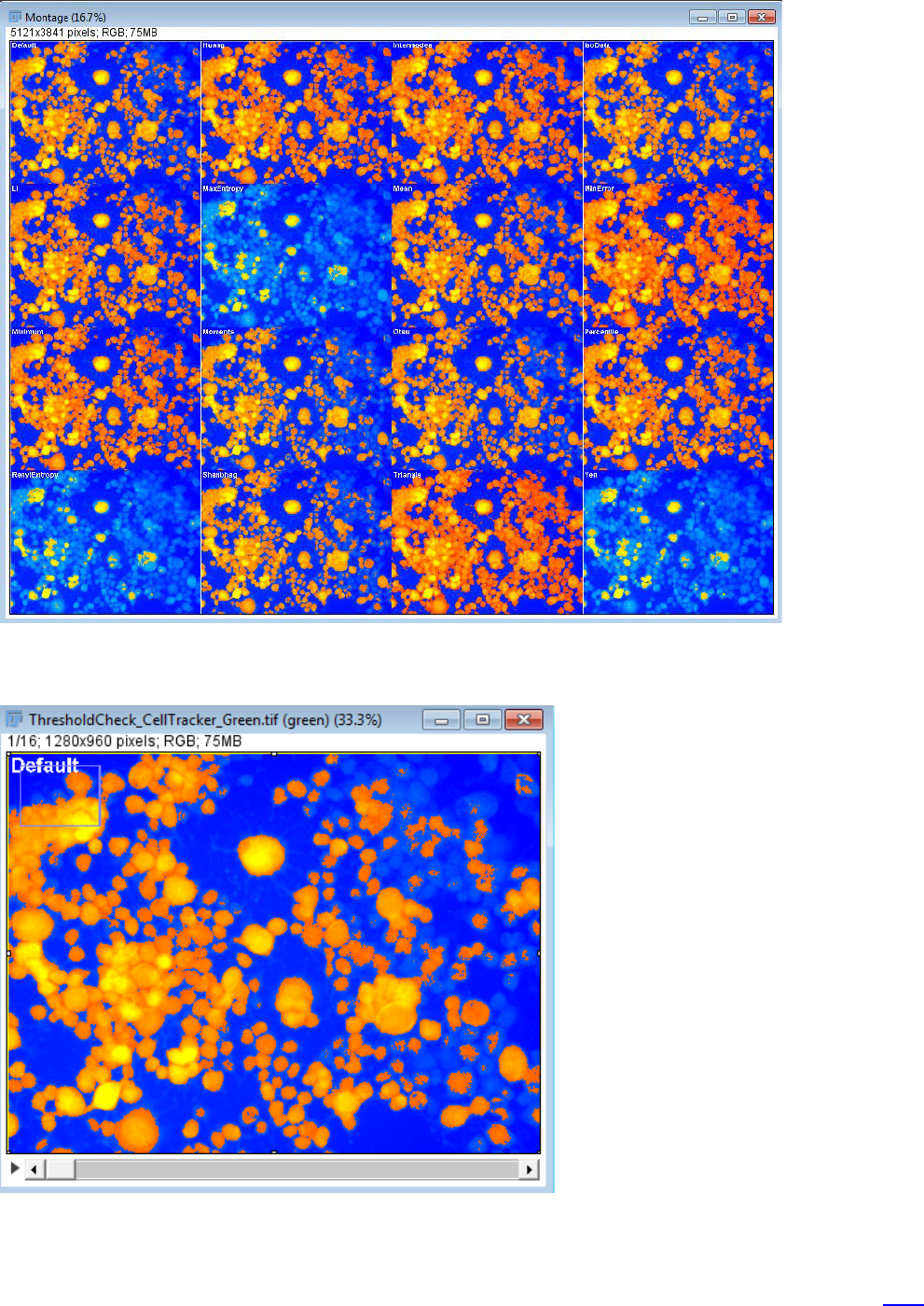
Image – Adjust – Auto Threshold;
Select from the options shown below;
The montage of the thresholded image is shown below;


25
Set the radius at a value that approximates the size of your objects. Use the Line Tool to make some initial
measurements of your objects if necessary. Please note that you need to specify whether your objects are
“White objects on black background” or not! Parameters 1 and 2 can be specified but only affect some of
the methods – check out the website for more information.

26
The results are shown as a montage – see below;
You can then select which method works best and use that for segmentation.

28
or view the individual colour map images which are provided as a stack that you can look through.
Adaptive Threshold plugin
–this plugin takes into account uneven background and varying intensity of staining. It’s available here
and
works only on 8-bit grayscale images. Block size should approximate your feature size.

29
A Mask can be created as shown below, which is then used for the analysis.

30
Image – Adjust - Color Threshold
- used for thresholding colour images for segmentation/analysis. There is a range of color spaces
available for use – Hue/Saturation/Brightness often works well for histology images. You can use
a Region of Interest to sample the hue to assist with the segmentation.
SHADING CORRECTION TOOLS
Process – Subtract Background
Uses Rolling Ball algorithm to smooth background variation. Choose the radius according to the size of
features. Select Light Background for brightfield/transmitted light colour images. Select Preview to see
the effect on your image immediately. Select Create Background if you don’t have a background image
and want to use the Calculator Plus plugin described below. It’s also helpful to select Preview and Create
Background to check whether you are using too high/low a radius. Structural detail shouldn’t be visible.
Process - Calculator Plus
Uses image and blank image together with a multiplication factor k1 of 255 for brightfield images as shown
below. If the corrected image looks too white, check the mean gray value of the background in your original
image and use that value for k1.

31
Process-Image-Calculator
allows you to do mathematical operations using 2 images – one must be a background image. One option
for creating a background image (if you don’t have one) is by blurring the original image, e.g. using a
Gaussian blur filter with a high Sigma (radius) value.
Shading Corrector Plugin
Available at: http://rsb.info.nih.gov/ij/plugins/shading-corrector.html
Requires a background image. Corrects for uneven illumination/pixel irregularities based on the mean pixel
value of the background image.
More….
If you want to read more about image correction for brightfield microscopy and requirements for acquiring
background images, etc., go to this great reference by Gabriel Landini that describes a number of methods
for background subtraction for transmitted light images (“How to correct background illumination in
brightfield microscopy”). Access the document through the ImageJ documentation Wiki here
32
FILTERS
Filters represent group processing rather than individual pixel operations. There are many things you can
do to change (e.g. improve) the look of the image or make analysis/thresholding easier, eg. sharpen edges,
reduce noise, subtract background, etc. The built-in filters available through the Process menu cover most
requirements but there are many more available to download and install.
Most filters are implemented using 3 x 3 spatial convolutions (linear filtering). In this procedure, the value of
each pixel in the selection is replaced with the weighted average of its 3 x 3 neighbourhood.
Smooth - Blurs (softens) the selected area. It can be used to reduce noise in an image or to
even out the greyscale in the area.
1 1 1
1 1 1
1 1 1
Sharpen - Increases contrast and accentuates detail in the selection, but may also accentuate
noise.
-1 -1 -1
-1 12 -1
-1 -1 -1
Rank filters rank (sort) the nine pixels in each 3 x 3 neighborhood and replace the pixel with the median,
minimum (lightest), or maximum (darkest) value, i.e. non-linear filtering. Use the Median filter to reduce
noise (Process – Filters – Median). This removes high values for the target/central pixel which might be
due to electronic noise. A lower value is inserted. This is repeated on the next pixel, etc. until the whole
image is treated. It gets rid of noise without causing significant blurring of the image.
Process – Noise -Despeckle is a median filter. It replaces each pixel with the median value in its 3 x 3
neighborhood. Median filters are good at removing salt and pepper noise. A simple way to see the
difference between smoothing filters such as Mean and Median filters is to add noise to an image and then
try each filter to see which works best. Noise can be added under Process – Noise – Add Noise.
The Process – Filters - Minimum filter erodes (shrinks) objects in grayscale images similar to the way
binary erosion shrinks objects in binary images. The Maximum filter dilates (expands) objects in grayscale
images similar to the way binary dilation expands objects in binary images.
Process – Filters - Unsharp Mask: sharpens up the image, good if you need extra contrast, usually better
than Sharpen as it has more control.

33
Process – Filters – Gaussian blur: smoothing filter – higher values (Sigma) provide more smoothing.
Process – Find edges – Sobel filter – finds edges in both X (horizontal) and Y (vertical) directions based
on differences in the local intensity gradient and combines them.
MORPHOLOGICAL OPERATIONS – BINARY IMAGES
Located under Process – Binary;
These operations are used to adjust binary images for analysis, either for direct measurements or for
editing Masks (a binary image that is going to be used to define the area/objects for analysis on another
image). The default options for these binary operations are that the objects of interest are white and the
background is black – check this under Process – Binary – Options. You can still use these options if you
have black objects on white background but in this case, make sure black background is not selected.

34
The Binary Options window is useful in demonstrating how the different processes work. You can turn on
the Preview option and select what you want to do and see the result. Iterations determines how many
times you want the operation to run and Count is how many connected pixels will be affected. These
options apply to all of these processes which are all available directly under the Process – Binary menu
and can be called by Macros.
The most common operators are:
• Erode/Dilate – take away/add pixels
• Open – Erode followed by Dilate – removes small outliers, smooths
• Close – Dilate followed by Erode – closes boundaries, smooths, can be used to fill holes
• Fill Holes – fills holes inside objects
• Watershed – splits adjoining particles – works best for rounded objects
A set of advanced Morphological Operators from Gabriel Landini are available here
.
ANALYZE MENU
This menu has all the analysis functions including the Set Measurements window, where you select what
parameters you want to measure. It also has the Analyze Particles option.

35
IMAGE – STACKS MENU
Allow you to work with stacks, (e.g. z series or time series data). You need to have a series (time, z, x-y) of
images which can be built into a stack. If you open the images as a numbered sequence, then they will
automatically be put into a stack in the correct order. The most commonly used options are available under
the Stk icon on the right hand side of the Tool Bar.
• Images to Stack: converts a set of 2D images that you have already opened into a stack.
• Stack to Images: splits the stack into individual images.
• Tools – range of editing options available including animation, etc
• Navigation: browsing images can be done using the > and < keys. The number of the current slice
and the total number of slices are displayed in the title bar. You can also use the slider bar in the
stack window.
• Make Montage: allows you to create a montage out of your stack images.
• Orthogonal view: provides orthogonal (or cross-section) views – XZ and YZ.
• Z Project: projection algorithms designed to render stacks into 2D projections.
• 3D Project: Allows you to project the stack and then rotate it.
• Label…Stack slices can be labelled as below;
Plugins - Volume Viewer
MOVIES
Time Stamper: allows you to add the time information onto your movie.
Zoomify: allows you to make a movie where you zoom in on a particular region.
Save As Movie: plugin that allows you to save with a wider variety of formats.
