Greenplum Database 4.2. Database Administrator Guide, Rev A01

Greenplum

Database 4.2

Database Administrator Guide

Rev: A01

EMC believes the information in this publication is accurate as of its publication date. The information is subject to

change without notice.

THE INFORMATION IN THIS PUBLICATION IS PROVIDED “AS IS.” EMC CORPORATION MAKES NO REPRESENTATIONS

OR WARRANTIES OF ANY KIND WITH RESPECT TO THE INFORMATION IN THIS PUBLICATION, AND SPECIFICALLY

DISCLAIMS IMPLIED WARRANTIES OF MERCHANTABILITY OR FITNESS FOR A PARTICULAR PURPOSE.

Use, copying, and distribution of any EMC software described in this publication requires an applicable software

license.

For the most up-to-date listing of EMC product names, see EMC Corporation Trademarks on EMC.com

All other trademarks used herein are the property of their respective owners.

Table of Contents iii

Greenplum Database DBA Guide 4.2 - Contents

Preface ............................................................................................... 1

About This Guide.............................................................................. 1

About the Greenplum Database Documentation Set ......................... 1

Document Conventions .................................................................... 2

Text Conventions ........................................................................ 2

Command Syntax Conventions ................................................... 3

Getting Support................................................................................ 3

Product information .................................................................... 3

Technical support........................................................................ 4

Chapter 1: Introduction to Greenplum ...................................... 5

Chapter 2: Accessing the Database ............................................ 6

Establishing a Database Session....................................................... 6

Supported Client Applications........................................................... 7

Greenplum Database Client Applications ..................................... 8

pgAdmin III for Greenplum Database ......................................... 9

Database Application Interfaces................................................ 12

Third-Party Client Tools ............................................................ 13

Troubleshooting Connection Problems ............................................ 14

Chapter 3: Configuring Client Authentication........................ 15

Allowing Connections to Greenplum Database ................................ 15

Editing the pg_hba.conf File...................................................... 16

Limiting Concurrent Connections .................................................... 17

Encrypting Client/Server Connections............................................. 18

Chapter 4: Managing Roles and Privileges ............................. 20

Security Best Practices for Roles and Privileges .............................. 20

Creating New Roles (Users)............................................................ 21

Altering Role Attributes............................................................. 21

Role Membership............................................................................ 22

Managing Object Privileges............................................................. 23

Simulating Row and Column Level Access Control..................... 24

Encrypting Data ............................................................................. 25

Encrypting Passwords..................................................................... 25

Enabling SHA-256 Encryption ................................................... 25

Time-based Authentication............................................................. 27

Chapter 5: Defining Database Objects..................................... 28

Creating and Managing Databases ................................................. 28

About Template Databases ....................................................... 28

Creating a Database ................................................................. 28

Viewing the List of Databases ................................................... 29

Altering a Database .................................................................. 29

Dropping a Database ................................................................ 30

Creating and Managing Tablespaces............................................... 30

Creating a Filespace.................................................................. 30

Moving the Location of Temporary or Transaction Files ............. 31

Creating a Tablespace............................................................... 32

Using a Tablespace to Store Database Objects.......................... 32

Table of Contents iv

Greenplum Database DBA Guide 4.2 - Contents

Viewing Existing Tablespaces and Filespaces ............................ 33

Dropping Tablespaces and Filespaces........................................ 33

Creating and Managing Schemas.................................................... 34

The Default “Public” Schema..................................................... 34

Creating a Schema ................................................................... 34

Schema Search Paths ............................................................... 34

Dropping a Schema .................................................................. 35

System Schemas ...................................................................... 35

Creating and Managing Tables........................................................ 35

Creating a Table ....................................................................... 35

Choosing the Table Storage Model.................................................. 39

Heap Storage............................................................................ 39

Append-Only Storage................................................................ 39

Choosing Row or Column-Oriented Storage .............................. 40

Using Compression (Append-Only Tables Only) ........................ 41

Checking the Compression and Distribution of an Append-Only Table

Support for Run-length Encoding .............................................. 43

Adding Column-level Compression ............................................ 43

Altering a Table ........................................................................ 48

Dropping a Table ...................................................................... 49

Partitioning Large Tables ................................................................ 50

Table Partitioning in Greenplum Database ................................ 51

Deciding on a Table Partitioning Strategy ................................. 51

Creating Partitioned Tables ....................................................... 52

Loading Partitioned Tables ........................................................ 55

Verifying Your Partition Strategy............................................... 56

Viewing Your Partition Design ................................................... 56

Maintaining Partitioned Tables .................................................. 57

Creating and Using Sequences ....................................................... 60

Creating a Sequence................................................................. 61

Using a Sequence ..................................................................... 61

Altering a Sequence.................................................................. 61

Dropping a Sequence................................................................ 61

Using Indexes in Greenplum Database ........................................... 61

Index Types.............................................................................. 63

Creating an Index ..................................................................... 64

Examining Index Usage ............................................................ 65

Managing Indexes..................................................................... 65

Dropping an Index .................................................................... 66

Creating and Managing Views......................................................... 66

Creating Views.......................................................................... 66

Dropping Views......................................................................... 66

Chapter 6: Managing Data .......................................................... 67

About Concurrency Control in Greenplum Database ....................... 67

Inserting Rows ............................................................................... 68

Updating Existing Rows .................................................................. 69

Deleting Rows ................................................................................ 69

Truncating a Table .................................................................... 69

Table of Contents v

Greenplum Database DBA Guide 4.2 - Contents

Working With Transactions ............................................................. 70

Transaction Isolation Levels...................................................... 70

Vacuuming the Database................................................................ 71

Configuring the Free Space Map ............................................... 72

Chapter 7: Loading and Unloading Data ................................. 73

Greenplum Database Loading Tools Overview ................................ 73

External Tables ......................................................................... 73

gpload

...................................................................................... 74

COPY

.......................................................................................... 74

Loading Data into Greenplum Database ......................................... 75

Accessing File-Based External Tables ........................................ 75

Using the Greenplum Parallel File Server (gpfdist) .................... 79

Using Hadoop Distributed File System (HDFS) Tables..................... 81

One-time HDFS Protocol Installation ......................................... 81

Creating and Using Web External Tables................................... 88

Loading Data Using an External Table....................................... 89

Loading and Writing Non-HDFS Custom Data............................ 89

Using a Custom Format ............................................................ 90

Creating External Tables - Examples......................................... 93

Handling Load Errors ................................................................ 95

Loading Data ............................................................................ 98

Optimizing Data Load and Query Performance .........................100

Unloading Data from Greenplum Database....................................100

Defining a File-Based Writable External Table ..........................101

Defining a Command-Based Writable External Web Table ........102

Unloading Data Using a Writable External Table.......................103

Unloading Data Using COPY .....................................................103

Transforming XML Data .................................................................104

XML Transformation Examples .................................................112

Formatting Data Files ....................................................................115

Formatting Rows......................................................................115

Formatting Columns ................................................................115

Representing NULL Values .......................................................116

Escaping ..................................................................................116

Character Encoding..................................................................117

Chapter 8: About Greenplum Query Processing...................118

Understanding Query Planning and Dispatch .................................118

Understanding Greenplum Query Plans .........................................119

Understanding Parallel Query Execution ........................................120

Chapter 9: Querying Data...........................................................122

Defining Queries............................................................................122

SQL Lexicon.............................................................................122

SQL Value Expressions.............................................................122

Using Functions and Operators......................................................132

Using Functions in Greenplum Database ..................................133

User-Defined Functions............................................................133

Built-in Functions and Operators..............................................134

Window Functions....................................................................136

Table of Contents vi

Greenplum Database DBA Guide 4.2 - Contents

Advanced Analytic Functions....................................................137

Query Performance .......................................................................149

Query Profiling ..............................................................................149

Reading EXPLAIN Output .........................................................149

Reading EXPLAIN ANALYZE Output ..........................................151

Examining Query Plans to Solve Problems ...............................152

Chapter 10: Managing Workload and Resources .................154

Overview of Greenplum Workload Management ............................154

How Resource Queues Work in Greenplum Database ...............154

Steps to Enable Workload Management ...................................158

Configuring Workload Management ...............................................159

Creating Resource Queues ............................................................160

Creating Queues with an Active Query Limit ............................160

Creating Queues with Memory Limits.......................................161

Creating Queues with a Query Planner Cost Limits...................161

Setting Priority Levels..............................................................162

Assigning Roles (Users) to a Resource Queue................................163

Removing a Role from a Resource Queue ................................163

Modifying Resource Queues...........................................................164

Altering a Resource Queue.......................................................164

Dropping a Resource Queue.....................................................164

Checking Resource Queue Status ..................................................164

Viewing Queued Statements and Resource Queue Status ........165

Viewing Resource Queue Statistics...........................................165

Viewing the Roles Assigned to a Resource Queue ....................165

Viewing the Waiting Queries for a Resource Queue ..................166

Clearing a Waiting Statement From a Resource Queue ............166

Viewing the Priority of Active Statements ................................167

Resetting the Priority of an Active Statement...........................167

Chapter 11: Defining Database Performance .......................168

Understanding the Performance Factors ........................................168

System Resources ...................................................................168

Workload .................................................................................168

Throughput..............................................................................168

Contention...............................................................................169

Optimization ............................................................................169

Determining Acceptable Performance ............................................169

Baseline Hardware Performance...............................................169

Performance Benchmarks ........................................................169

Chapter 12: Common Causes of Performance Issues.........170

Identifying Hardware and Segment Failures ..................................170

Managing Workload.......................................................................171

Avoiding Contention ......................................................................171

Maintaining Database Statistics .....................................................171

Identifying Statistics Problems in Query Plans .........................171

Tuning Statistics Collection ......................................................172

Optimizing Data Distribution .........................................................172

Optimizing Your Database Design..................................................172

Table of Contents vii

Greenplum Database DBA Guide 4.2 - Contents

Greenplum Database Maximum Limits .....................................173

Chapter 13: Investigating a Performance Problem ............174

Checking System State .................................................................174

Checking Database Activity ...........................................................174

Checking for Active Sessions (Workload) .................................174

Checking for Locks (Contention) ..............................................174

Checking Query Status and System Utilization.........................175

Troubleshooting Problem Queries ..................................................175

Investigating Error Messages ........................................................175

Gathering Information for Greenplum Support.........................176

About This Guide 1

Greenplum Database DBA Guide 4.2 – Preface

Preface

This guide provides information for database administrators and database superusers

responsible for administering a Greenplum Database system.

• About This Guide

• Document Conventions

• Getting Support

About This Guide

This guide explains how clients connect to a Greenplum Database system, how to

configure access control and workload management, perform basic administration

tasks such as defining database objects, loading and unloading data, writing queries,

and managing data, and provides guidance on identifying and troubleshooting

common performance issues.

This guide assumes knowledge of database management systems, database

administration, and structured query language (SQL).

Because Greenplum Database is based on PostgreSQL 8.2.15, this guide assumes

some familiarity with PostgreSQL. References to PostgreSQL documentation are

provided for features that are similar to those in Greenplum Database.

About the Greenplum Database Documentation Set

As of Release 4.2.3, the Greenplum Database documentation set consists of the

following guides.

Table 0.1

Greenplum Database documentation set

Guide Name Description

Greenplum Database Database

Administrator Guide

Every day DBA tasks such as configuring access control and

workload management, writing queries, managing data,

defining database objects, and performance troubleshooting.

Greenplum Database System

Administrator Guide

Describes the Greenplum Database architecture and concepts

such as parallel processing, and system administration tasks

for Greenplum Database such as configuring the server,

monitoring system activity, enabling high-availability, backing

up and restoring databases, and expanding the system.

Greenplum Database Reference

Guide

Reference information for Greenplum Database systems: SQL

commands, system catalogs, environment variables, character

set support, datatypes, the Greenplum MapReduce

specification, postGIS extension, server parameters, the

gp_toolkit administrative schema, and SQL 2008 support.

Greenplum Database Utility

Guide

Reference information for command-line utilities, client

programs, and Oracle compatibility functions.

Greenplum Database

Installation Guide

Information and instructions for installing and initializing a

Greenplum Database system.

Document Conventions 2

Greenplum Database DBA Guide 4.2 – Preface

Document Conventions

The following conventions are used throughout the Greenplum Database

documentation to help you identify certain types of information.

• Text Conventions

• Command Syntax Conventions

Text Conventions

Table 0.2

Text Conventions

Text Convention Usage Examples

bold Button, menu, tab, page, and field

names in GUI applications

Click Cancel to exit the page without

saving your changes.

italics New terms where they are defined

Database objects, such as schema,

table, or columns names

The master instance is the

postgres

process that accepts client

connections.

Catalog information for Greenplum

Database resides in the pg_catalog

schema.

monospace

File names and path names

Programs and executables

Command names and syntax

Parameter names

Edit the

postgresql.conf

file.

Use

gpstart

to start Greenplum

Database.

monospace italics

Variable information within file

paths and file names

Variable information within

command syntax

/home/gpadmin

config_file

COPY

tablename

FROM

filename

monospace bold

Used to call attention to a particular

part of a command, parameter, or

code snippet.

Change the host name, port, and

database name in the JDBC

connection URL:

jdbc:postgresql://host:5432/m

ydb

UPPERCASE

Environment variables

SQL commands

Keyboard keys

Make sure that the Java

/bin

directory is in your

$PATH

SELECT * FROM

my_table

;

Press

CTRL+C

to escape.

Getting Support 3

Greenplum Database DBA Guide 4.2 – Preface

Command Syntax Conventions

Table 0.3

Command Syntax Conventions

Text Convention Usage Examples

{ }

Within command syntax, curly

braces group related command

options. Do not type the curly

braces.

FROM { '

filename

' | STDIN }

[ ]

Within command syntax, square

brackets denote optional

arguments. Do not type the

brackets.

TRUNCATE [ TABLE ]

name

...

Within command syntax, an ellipsis

denotes repetition of a command,

variable, or option. Do not type the

ellipsis.

DROP TABLE

name

[, ...]

Within command syntax, the pipe

symbol denotes an “OR”

relationship. Do not type the pipe

symbol.

VACUUM [ FULL | FREEZE ]

$ system_command

# root_system_command

=> gpdb_command

=# su_gpdb_command

Denotes a command prompt - do

not type the prompt symbol.

and

denote terminal command

prompts.

and

denote

Greenplum Database interactive

program command prompts (

psql

gpssh

, for example).

$ createdb mydatabase

# chown gpadmin -R /datadir

=> SELECT * FROM mytable;

=# SELECT * FROM pg_database;

Getting Support

EMC support, product, and licensing information can be obtained as follows.

Product information

For documentation, release notes, software updates, or for information about EMC

products, licensing, and service, go to the EMC Powerlink website (registration

required) at:

http://Powerlink.EMC.com

Getting Support 4

Greenplum Database DBA Guide 4.2 – Preface

Technical support

For technical support, go to Powerlink and choose Support. On the Support page, you

will see several options, including one for making a service request. Note that to open

a service request, you must have a valid support agreement. Please contact your EMC

sales representative for details about obtaining a valid support agreement or with

questions about your account.

Greenplum Database DBA Guide 4.2 – Chapter 1: Introduction to Greenplum

Introduction to Greenplum

Greenplum Database is a massively parallel processing (MPP) database server based

on PostgreSQL open-source technology. MPP (also known as a shared nothing

architecture) refers to systems with two or more processors that cooperate to carry out

an operation - each processor with its own memory, operating system and disks.

Greenplum uses this high-performance system architecture to distribute the load of

multi-terabyte data warehouses, and can use all of a system’s resources in parallel to

process a query.

Greenplum Database is essentially several PostgreSQL database instances acting

together as one cohesive database management system (DBMS). It is based on

PostgreSQL 8.2.15, and in most cases is very similar to PostgreSQL with regard to

SQL support, features, configuration options, and end-user functionality. Database

users interact with Greenplum Database as they would a regular PostgreSQL DBMS.

The internals of PostgreSQL have been modified or supplemented to support the

parallel structure of Greenplum Database. For example, the system catalog, query

planner, optimizer, query executor, and transaction manager components have been

modified and enhanced to be able to execute queries simultaneously across all of the

parallel PostgreSQL database instances. The Greenplum interconnect (the networking

layer) enables communication between the distinct PostgreSQL instances and allows

the system to behave as one logical database.

Greenplum Database also includes features designed to optimize PostgreSQL for

business intelligence (BI) workloads. For example, Greenplum has added parallel data

loading (external tables), resource management, query optimizations, and storage

enhancements, which are not found in standard PostgreSQL. Many features and

optimizations developed by Greenplum make their way into the PostgreSQL

community. For example, table partitioning is a feature first developed by Greenplum,

and it is now in standard PostgreSQL.

Establishing a Database Session 6

Greenplum Database DBA Guide 4.2 – Chapter 2: Accessing the Database

Accessing the Database

This chapter explains the various client tools you can use to connect to Greenplum

Database, and how to establish a database session. It contains the following topics:

• Establishing a Database Session

• Supported Client Applications

• Troubleshooting Connection Problems

Establishing a Database Session

Users can connect to Greenplum Database using a PostgreSQL-compatible client

program, such as

psql

. Users and administrators always connect to Greenplum

Database through the master - the segments cannot accept client connections.

In order to establish a connection to the Greenplum Database master, you will need to

know the following connection information and configure your client program

accordingly.

Table 2.1

Connection Parameters

Connection Parameter Description Environment Variable

Application name The application name that is

connecting to the database. The

default value, held in the

application_name

connection

parameter is psql.

$PGAPPNAME

Database name The name of the database to which

you want to connect. For a newly

initialized system, use the

template1

database to connect

for the first time.

$PGDATABASE

Host name The host name of the Greenplum

Database master. The default host

is the local host.

$PGHOST

Supported Client Applications 7

Greenplum Database DBA Guide 4.2 – Chapter 2: Accessing the Database

Supported Client Applications

Users can connect to Greenplum Database using various client applications:

• A number of Greenplum Database Client Applications are provided with your

Greenplum installation. The

psql

client application provides an interactive

command-line interface to Greenplum Database.

• pgAdmin III for Greenplum Database is an enhanced version of the popular

management tool pgAdmin III. Since version 1.10.0, the pgAdmin III client

available from PostgreSQL Tools includes support for Greenplum-specific

features. Installation packages are available for download from the

pgAdmin

download site.

• Using standard Database Application Interfaces, such as ODBC and JDBC, users

can create their own client applications that interface to Greenplum Database.

Because Greenplum Database is based on PostgreSQL, it uses the standard

PostgreSQL database drivers.

• Most Third-Party Client Tools that use standard database interfaces, such as

ODBC and JDBC, can be configured to connect to Greenplum Database.

Port The port number that the

Greenplum Database master

instance is running on. The default

is 5432.

$PGPORT

User name The database user (role) name to

connect as. This is not necessarily

the same as your OS user name.

Check with your Greenplum

administrator if you are not sure

what you database user name is.

Note that every Greenplum

Database system has one

superuser account that is created

automatically at initialization time.

This account has the same name

as the OS name of the user who

initialized the Greenplum system

(typically

gpadmin

$PGUSER

Table 2.1

Connection Parameters

Connection Parameter Description Environment Variable

Supported Client Applications 8

Greenplum Database DBA Guide 4.2 – Chapter 2: Accessing the Database

Greenplum Database Client Applications

Greenplum Database comes installed with a number of client applications located in

$GPHOME/bin

of your Greenplum Database master host installation. The following

are the most commonly used client applications:

Table 2.2

Commonly used client applications

Name Usage

createdb

create a new database

createlang

define a new procedural language

createuser

define a new database role

dropdb

remove a database

droplang

remove a procedural language

dropuser

remove a role

psql

PostgreSQL interactive terminal

reindexdb

reindex a database

vacuumdb

garbage-collect and analyze a database

When using these client applications, you must connect to a database through the

Greenplum master instance. You will need to know the name of your target database,

the host name and port number of the master, and what database user name to connect

as. This information can be provided on the command-line using the options

-d

-h

-p

, and

-U

respectively. If an argument is found that does not belong to any option, it

will be interpreted as the database name first.

All of these options have default values which will be used if the option is not

specified. The default host is the local host. The default port number is 5432. The

default user name is your OS system user name, as is the default database name. Note

that OS user names and Greenplum Database user names are not necessarily the same.

If the default values are not correct, you can set the environment variables

PGDATABASE

PGHOST

PGPORT

, and

PGUSER

to the appropriate values, or use a

psql

~/.pgpass

file to contain frequently-used passwords. For information about

Greenplum Database environment variables, see the Greenplum Database Reference

Guide. For information about psql, see the Greenplum Database Utility Guide.

Connecting with psql

Depending on the default values used or the environment variables you have set, the

following examples show how to access a database via

psql

$ psql -d gpdatabase -h master_host -p 5432 -U

gpadmin

$ psql gpdatabase

$ psql

If a user-defined database has not yet been created, you can access the system by

connecting to the

template1

database. For example:

Supported Client Applications 9

Greenplum Database DBA Guide 4.2 – Chapter 2: Accessing the Database

$ psql template1

After connecting to a database,

psql

provides a prompt with the name of the database

to which

psql

is currently connected, followed by the string

(or

if you are the

database superuser). For example:

gpdatabase=>

At the prompt, you may type in SQL commands. A SQL command must end with a

;

(semicolon) in order to be sent to the server and executed. For example:

=> SELECT * FROM mytable;

See the Greenplum Reference Guide for information about using the

psql

client

application and SQL commands and syntax.

pgAdmin III for Greenplum Database

If you prefer a graphic interface, use pgAdmin III for Greenplum Database. This GUI

client supports PostgreSQL databases with all standard pgAdmin III features, while

adding support for Greenplum-specific features.

pgAdmin III for Greenplum Database supports the following Greenplum-specific

features:

• External tables

• Append-only tables, including compressed append-only tables

• Table partitioning

• Resource queues

• Graphical

EXPLAIN ANALYZE

• Greenplum server configuration parameters

Supported Client Applications 10

Greenplum Database DBA Guide 4.2 – Chapter 2: Accessing the Database

Figure 2.1

Greenplum Options in pgAdmin III

Installing pgAdmin III for Greenplum Database

The installation package for pgAdmin III for Greenplum Database is available for

download from the official pgAdmin III download site (http://www.pgadmin.org).

Installation instructions are included in the installation package.

Documentation for pgAdmin III for Greenplum Database

For general help on the features of the graphical interface, select Help contents from

the Help menu.

For help with Greenplum-specific SQL support, select Greenplum Database Help

from the Help menu. If you have an active internet connection, you will be directed to

online Greenplum SQL reference documentation. Alternately, you can install the

Greenplum Client Tools package. This package contains SQL reference

documentation that is accessible to the help links in pgAdmin III.

Performing Administrative Tasks with pgAdmin III

This section highlights two of the many Greenplum Database administrative tasks you

can perform with pgAdmin III: editing the server configuration, and viewing a

graphical representation of a query plan.

Supported Client Applications 11

Greenplum Database DBA Guide 4.2 – Chapter 2: Accessing the Database

Editing Server Configuration

The pgAdmin III interface provides two ways to update the server configuration in

postgresql.conf

: locally, through the File menu, and remotely on the server

through the Tools menu. Editing the server configuration remotely may be more

convenient in many cases, because it does not require you to upload or copy

postgresql.conf.

To edit server configuration remotely

1. Connect to the server whose configuration you want to edit. If you are connected

to multiple servers, make sure that the correct server is highlighted in the object

browser in the left pane.

2. Select Tools > Server Configuration > postgresql.conf. The Backend

Configuration Editor opens, displaying the list of available and enabled server

configuration parameters.

3. Locate the parameter you want to edit, and double click on the entry to open the

Configuration settings dialog.

4. Enter the new value for the parameter, or select/deselect Enabled as desired and

click OK.

5. If the parameter can be enabled by reloading server configuration, click the green

reload icon, or select File > Reload server. Many parameters require a full restart

of the server.

Viewing a Graphical Query Plan

Using the pgAdmin III query tool, you can run a query with EXPLAIN to view the

details of the query plan. The output includes details about operations unique to

Greenplum distributed query processing such as plan slices and motions between

segments. You can view a graphical depiction of the plan as well as the text-based data

output.

To view a graphical query plan

1. With the correct database highlighted in the object browser in the left pane, select

Tools > Query tool.

2. Enter the query by typing in the SQL Editor, dragging objects into the Graphical

Query Builder, or opening a file.

3. Select Query > Explain options and verify the following options:

• Verbose — this must be deselected if you want to view a graphical depiction

of the query plan

• Analyze — select this option if you want to run the query in addition to

viewing the plan

4. Trigger the operation by clicking the Explain query option at the top of the pane,

or by selecting Query > Explain.

The query plan displays in the Output pane at the bottom of the screen. Select the

Explain tab to view the graphical output. For example:

Supported Client Applications 12

Greenplum Database DBA Guide 4.2 – Chapter 2: Accessing the Database

Figure 2.2

Graphical Query Plan in pgAdmin III

Database Application Interfaces

You may want to develop your own client applications that interface to Greenplum

Database. PostgreSQL provides a number of database drivers for the most commonly

used database application programming interfaces (APIs), which can also be used

with Greenplum Database. These drivers are not packaged with the Greenplum

Database base distribution. Each driver is an independent PostgreSQL development

project and must be downloaded, installed and configured to connect to Greenplum

Database. The following drivers are available:

Table 2.3

Greenplum Database Interfaces

API PostgreSQL Driver Download Link

ODBC pgodbc Available in the Greenplum Database

Connectivity package, which can be

downloaded from the EMC Download

Center.

JDBC pgjdbc Available in the Greenplum Database

Connectivity package, which can be

downloaded from the EMC Download

Center.

Perl DBI pgperl http://gborg.postgresql.org/project/pgperl

Python DBI pygresql http://www.pygresql.org

Supported Client Applications 13

Greenplum Database DBA Guide 4.2 – Chapter 2: Accessing the Database

General instructions for accessing a Greenplum Database with an API are:

1. Download your programming language platform and respective API from the

appropriate source. For example, you can get the Java development kit (JDK) and

JDBC API from Sun.

2. Write your client application according to the API specifications. When

programming your application, be aware of the SQL support in Greenplum

Database so you do not include any unsupported SQL syntax. See the Greenplum

Database Reference Guide for more information.

Download the appropriate PostgreSQL driver and configure connectivity to your

Greenplum Database master instance. Greenplum provides a client tools package that

contains the supported database drivers for Greenplum Database. Download the client

tools package and documentation from the

EMC Download Center.

Third-Party Client Tools

Most third-party extract-transform-load (ETL) and business intelligence (BI) tools use

standard database interfaces, such as ODBC and JDBC, and can be configured to

connect to Greenplum Database. Greenplum has worked with the following tools on

previous customer engagements and is in the process of becoming officially certified:

• Business Objects

• Microstrategy

• Informatica Power Center

• Microsoft SQL Server Integration Services (SSIS) and Reporting Services (SSRS)

• Ascential Datastage

• SAS

• Cognos

Greenplum Professional Services can assist users in configuring their chosen

third-party tool for use with Greenplum Database.

Troubleshooting Connection Problems 14

Greenplum Database DBA Guide 4.2 – Chapter 2: Accessing the Database

Troubleshooting Connection Problems

A number of things can prevent a client application from successfully connecting to

Greenplum Database. This section explains some of the common causes of connection

problems and how to correct them.

Table 2.4

Common connection problems

Problem Solution

pg_hba.conf

entry for

host or user

To enable Greenplum Database to accept remote client connections,

you must configure your Greenplum Database master instance so

that connections are allowed from the client hosts and database

users that will be connecting to Greenplum Database. This is done by

adding the appropriate entries to the

pg_hba.conf

configuration file

(located in the master instance’s data directory). For more detailed

information, see

“Allowing Connections to Greenplum Database” on

page

15.

Greenplum Database is not

running

If the Greenplum Database master instance is down, users will not be

able to connect. You can verify that the Greenplum Database system

is up by running the

gpstate

utility on the Greenplum master host.

Network problems

Interconnect timeouts

If users connect to the Greenplum master host from a remote client,

network problems can prevent a connection (for example, DNS host

name resolution problems, the host system is down, and so on.). To

ensure that network problems are not the cause, connect to the

Greenplum master host from the remote client host. For example:

ping

hostname

If the system cannot resolve the host names and IP addresses of the

hosts involved in Greenplum Database, queries and connections will

fail. For some operations, connections to the Greenplum Database

master use

localhost

and others use the actual host name, so you

must be able to resolve both. If you encounter this error, first make

sure you can connect to each host in your Greenplum Database

array from the master host over the network. In the

/etc/hosts

file

of the master and all segments, make sure you have the correct host

names and IP addresses for all hosts involved in the Greenplum

Database array. The

127.0.0.1

IP must resolve to

localhost

Too many clients already By default, Greenplum Database is configured to allow a maximum of

250 concurrent user connections on the master and 750 on a

segment. A connection attempt that causes that limit to be exceeded

will be refused. This limit is controlled by the

max_connections

parameter in the

postgresql.conf

configuration file of the

Greenplum Database master. If you change this setting for the

master, you must also make appropriate changes at the segments.

Allowing Connections to Greenplum Database 15

Greenplum Database DBA Guide 4.2 – Chapter 3: Configuring Client Authentication

Configuring Client Authentication

When a Greenplum Database system is first initialized, the system contains one

predefined superuser role. This role will have the same name as the operating system

user who initialized the Greenplum Database system. This role is referred to as

gpadmin

. By default, the system is configured to only allow local connections to the

database from the

gpadmin

role. If you want to allow any other roles to connect, or if

you want to allow connections from remote hosts, you have to configure Greenplum

Database to allow such connections. This chapter explains how to configure client

connections and authentication to Greenplum Database.

• Allowing Connections to Greenplum Database

• Limiting Concurrent Connections

Allowing Connections to Greenplum Database

Client access and authentication is controlled by the standard PostgreSQL host-based

authentication file, pg_hba.conf. In Greenplum Database, the

pg_hba.conf

file of the

master instance controls client access and authentication to your Greenplum system.

Greenplum segments have

pg_hba.conf

files that are configured to allowonly client

connections from the master host and never accept client connections. Do not alter the

pg_hba.conf

file on your segments.

See The pg_hba.conf File in the PostgreSQL documentation for more information.

The general format of the

pg_hba.conf

file is a set of records, one per line.

Greenplum ignores blank lines and any text after the

comment character. A record

consists of a number of fields that are separated by spaces and/or tabs. Fields can

contain white space if the field value is quoted. Records cannot be continued across

lines. Each remote client access record has the following format:

host database role CIDR-address authentication-method

Each UNIX-domain socket access record has the following format:

local database role authentication-method

The following table describes meaning of each field.

Table 3.1

pg_hba.conf Fields

Field Description

local Matches connection attempts using UNIX-domain sockets. Without a

record of this type, UNIX-domain socket connections are disallowed.

host Matches connection attempts made using TCP/IP. Remote TCP/IP

connections will not be possible unless the server is started with an

appropriate value for the listen_addresses server configuration

parameter.

hostssl Matches connection attempts made using TCP/IP, but only when the

connection is made with SSL encryption. SSL must be enabled at

server start time by setting the ssl configuration parameter

Allowing Connections to Greenplum Database 16

Greenplum Database DBA Guide 4.2 – Chapter 3: Configuring Client Authentication

Editing the pg_hba.conf File

This example shows how to edit the

pg_hba.conf

file of the master to allow remote

client access to all databases from all roles using encrypted password authentication.

Note: For a more secure system, consider removing all connections that use trust

authentication from your master

pg_hba.conf

. Trust authentication means the role

is granted access without any authentication, therefore bypassing all security.

Replace trust entries with ident authentication if your system has an ident service

available.

Editing pg_hba.conf

1. Open the file

$MASTER_DATA_DIRECTORY/pg_hba.conf

in a text editor.

hostnossl Matches connection attempts made over TCP/IP that do not use

SSL.

database

Specifies which database names this record matches. The value

all

specifies that it matches all databases. Multiple database names can

be supplied by separating them with commas. A separate file

containing database names can be specified by preceding the file

name with @.

role Specifies which database role names this record matches. The value

all

specifies that it matches all roles. If the specified role is a group

and you want all members of that group to be included, precede the

role name with a +. Multiple role names can be supplied by

separating them with commas. A separate file containing role names

can be specified by preceding the file name with @.

CIDR-address Specifies the client machine IP address range that this record

matches. It contains an IP address in standard dotted decimal

notation and a CIDR mask length. IP addresses can only be

specified numerically, not as domain or host names. The mask length

indicates the number of high-order bits of the client IP address that

must match. Bits to the right of this must be zero in the given IP

address. There must not be any white space between the IP

address, the /, and the CIDR mask length.

Typical examples of a CIDR-address are 172.20.143.89/32 for a

single host, or 172.20.143.0/24 for a small network, or 10.6.0.0/16 for

a larger one. To specify a single host, use a CIDR mask of 32 for

IPv4 or 128 for IPv6. In a network address, do not omit trailing

zeroes.

IP-address

IP-mask

These fields can be used as an alternative to the CIDR-address

notation. Instead of specifying the mask length, the actual mask is

specified in a separate column. For example, 255.0.0.0 represents

an IPv4 CIDR mask length of 8, and 255.255.255.255 represents a

CIDR mask length of 32. These fields only apply to host, hostssl, and

hostnossl records.

authentication-method Specifies the authentication method to use when connecting.

Greenplum supports the authentication methods supported by

Postgre 9.0.

Table 3.1

pg_hba.conf Fields

Field Description



Limiting Concurrent Connections 17

Greenplum Database DBA Guide 4.2 – Chapter 3: Configuring Client Authentication

2. Add a line to the file for each type of connection you want to allow. Records are

read sequentially, so the order of the records is significant. Typically, earlier

records will have tight connection match parameters and weaker authentication

methods, while later records will have looser match parameters and stronger

authentication methods. For example:

# allow the gpadmin user local access to all databases

# using ident authentication

local all gpadmin ident sameuser

host all gpadmin 127.0.0.1/32 ident

host all gpadmin ::1/128 ident

# allow the 'dba' role access to any database from any

# host with IP address 192.168.x.x and use md5 encrypted

# passwords to authenticate the user

# Note that to use SHA-256 encryption, replace

md5

with

password

in the line below

host all dba 192.168.0.0/32 md5

# allow all roles access to any database from any

# host and use ldap to authenticate the user. Greenplum role

# names must match the LDAP common name.

host all all 192.168.0.0/32 ldap ldapserver=usldap1

ldapport=1389 ldapprefix="cn="

ldapsuffix=",ou=People,dc=company,dc=com"

3. Save and close the file.

4. Reload the

pg_hba.conf

configuration file for your changes to take effect:

$ gpstop -u

Note: Note that you can also control database access by setting object privileges as

described in “Managing Object Privileges” on page 33. The

pg_hba.conf

file just

controls who can initiate a database session and how those connections are

authenticated.

Limiting Concurrent Connections

To limit the number of active concurrent sessions to your Greenplum Database

system, you can configure the

max_connections

server configuration parameter. This

is a local parameter, meaning that you must set it in the

postgresql.conf

file of the

master, the standby master, and each segment instance (primary and mirror). The

value of

max_connections on segments must be 5-10 times the value on the master.

When you set

max_connections

, you must also set the dependent parameter

max_prepared_transactions

. This value must be at least as large as the value of

max_connections

on the master, and segment instances should be set to the same

value as the master.

For example:

$MASTER_DATA_DIRECTORY/postgresql.conf

(including standby master):



Encrypting Client/Server Connections 18

Greenplum Database DBA Guide 4.2 – Chapter 3: Configuring Client Authentication

max_connections=100

max_prepared_transactions=100

SEGMENT_DATA_DIRECTORY

/postgresql.conf

for all segment instances:

max_connections=500

max_prepared_transactions=100

To change the number of allowed connections

1. Stop your Greenplum Database system:

$ gpstop

2. On your master host, edit

$MASTER_DATA_DIRECTORY/postgresql.conf

and

change the following two parameters:

max_connections

(the number of active user sessions you want to allow plus the

number of

superuser_reserved_connections

)

max_prepared_transactions

(must be greater than or equal to

max_connections

)

3. On each segment instance, edit

SEGMENT_DATA_DIRECTORY

/postgresql.conf

and and change the following two parameters:

max_connections

(must be 5-10 times the value on the master)

max_prepared_transactions

(must be equal to the value on the master)

4. Restart your Greenplum Database system:

$ gpstart

Note: Raising the values of these parameters may cause Greenplum Database to

request more shared memory. To mitigate this effect, consider decreasing

other memory-related parameters such as

gp_cached_segworkers_threshold

Encrypting Client/Server Connections

Greenplum Database has native support for SSL connections between the client and

the master server. SSL connections prevent third parties from snooping on the packets,

and also prevent man-in-the-middle attacks. SSL should be used whenever the client

connection goes through an insecure link, and must be used whenever client certificate

authentication is used.

To enable SSL requires that OpenSSL be installed on both the client and the master

server systems. Greenplum can be started with SSL enabled by setting the server

configuration parameter

ssl=on

in the master

postgresql.conf

. When starting in

SSL mode, the server will look for the files

server.key

(server private key) and

server.crt

(server certificate) in the master data directory. These files must be set

up correctly before an SSL-enabled Greenplum system can start.

Important: Do not protect the private key with a passphrase. The server

does not prompt for a passphrase for the private key, and the database

startup fails with an error if one is required.



Encrypting Client/Server Connections 19

Greenplum Database DBA Guide 4.2 – Chapter 3: Configuring Client Authentication

A self-signed certificate can be used for testing, but a certificate signed by a certificate

authority (CA) should be used in production, so the client can verify the identity of the

server. Either a global or local CA can be used. If all the clients are local to the

organization, a local CA is recommended.

Creating a Self-signed Certificate without a Passphrase for Testing Only

To create a quick self-signed certificate for the server for testing, use the following

OpenSSL command:

# openssl req -new -text -out server.req

Fill out the information that openssl asks for. Be sure to enter the local host name as

Common Name. The challenge password can be left blank.

The program will generate a key that is passphrase protected, and does not accept a

passphrase that is less than four characters long.

To use this certificate with Greenplum Database, remove the passphrase with the

following commands:

# openssl rsa -in privkey.pem -out server.key

# rm privkey.pem

Enter the old passphrase when prompted to unlock the existing key.

Then, enter the following command to turn the certificate into a self-signed certificate

and to copy the key and certificate to a location where the server will look for them.

# openssl req -x509 -in server.req -text -key server.key -out server.crt

Finally, change the permissions on the key with the following command. The server

will reject the file if the permissions are less restrictive than these.

# chmod og-rwx server.key

For more details on how to create your server private key and certificate, refer to the

OpenSSL documentation.

Security Best Practices for Roles and Privileges 20

Greenplum Database DBA Guide 4.2 – Chapter 4: Managing Roles and Privileges

Managing Roles and Privileges

Greenplum Database manages database access permissions using the concept of roles.

The concept of roles subsumes the concepts of users and groups. A role can be a

database user, a group, or both. Roles can own database objects (for example, tables)

and can assign privileges on those objects to other roles to control access to the

objects. Roles can be members of other roles, thus a member role can inherit the

object privileges of its parent role.

Every Greenplum Database system contains a set of database roles (users and groups).

Those roles are separate from the users and groups managed by the operating system

on which the server runs. However, for convenience you may want to maintain a

relationship between operating system user names and Greenplum Database role

names, since many of the client applications use the current operating system user

name as the default.

In Greenplum Database, users log in and connect through the master instance, which

then verifies their role and access privileges. The master then issues out commands to

the segment instances behind the scenes as the currently logged in role.

Roles are defined at the system level, meaning they are valid for all databases in the

system.

In order to bootstrap the Greenplum Database system, a freshly initialized system

always contains one predefined superuser role (also referred to as the system user).

This role will have the same name as the operating system user that initialized the

Greenplum Database system. Customarily, this role is named

gpadmin

. In order to

create more roles you first have to connect as this initial role.

Security Best Practices for Roles and Privileges

• Secure the gpadmin system user. Greenplum requires a UNIX user id to install

and initialize the Greenplum Database system. This system user is referred to as

gpadmin

in the Greenplum documentation. This

gpadmin

user is the default

database superuser in Greenplum Database, as well as the file system owner of the

Greenplum installation and its underlying data files. This default administrator

account is fundamental to the design of Greenplum Database. The system cannot

run without it, and there is no way to limit the access of this gpadmin user id. Use

roles to manage who has access to the database for specific purposes. You should

only use the

gpadmin

account for system maintenance tasks such as expansion

and upgrade. Anyone who logs on to a Greenplum host as this user id can read,

alter or delete any data; including system catalog data and database access rights.

Therefore, it is very important to secure the gpadmin user id and only provide

access to essential system administrators. Administrators should only log in to

Greenplum as

gpadmin

when performing certain system maintenance tasks (such

as upgrade or expansion). Database users should never log on as

gpadmin

, and

ETL or production workloads should never run as

gpadmin

Creating New Roles (Users) 21

Greenplum Database DBA Guide 4.2 – Chapter 4: Managing Roles and Privileges

• Assign a distinct role to each user that logs in. For logging and auditing

purposes, each user that is allowed to log in to Greenplum Database should be

given their own database role. For applications or web services, consider creating

a distinct role for each application or service. See

“Creating New Roles (Users)”

on page 21.

• Use groups to manage access privileges. See “Role Membership” on page 22.

• Limit users who have the SUPERUSER role attribute. Roles that are

superusers bypass all access privilege checks in Greenplum Database, as well as

resource queuing. Only system administrators should be given superuser rights.

See

“Altering Role Attributes” on page 21.

Creating New Roles (Users)

A user-level role is considered to be a database role that can log in to the database and

initiate a database session. Therefore, when you create a new user-level role using the

CREATE ROLE

command, you must specify the

privilege. For example:

=# CREATE ROLE jsmith WITH LOGIN;

A database role may have a number of attributes that define what sort of tasks that role

can perform in the database. You can set these attributes when you create the role, or

later using the

ALTER ROLE

command. See Table 4.1, “Role Attributes” on page 21

for a description of the role attributes you can set.

Altering Role Attributes

A database role may have a number of attributes that define what sort of tasks that role

can perform in the database.

Table 4.1

Role Attributes

Attributes Description

SUPERUSER | NOSUPERUSER Determines if the role is a superuser. You must yourself be a

superuser to create a new superuser. NOSUPERUSER is the default.

CREATEDB | NOCREATEDB Determines if the role is allowed to create databases. NOCREATEDB

is the default.

CREATEROLE | NOCREATEROLE Determines if the role is allowed to create and manage other roles.

NOCREATEROLE is the default.

INHERIT | NOINHERIT Determines whether a role inherits the privileges of roles it is a

member of. A role with the INHERIT attribute can automatically use

whatever database privileges have been granted to all roles it is

directly or indirectly a member of. INHERIT is the default.

attribute are useful for managing database privileges (groups).

NOLOGIN is the default.

CONNECTION LIMIT connlimit If role can log in, this specifies how many concurrent connections the

role can make. -1 (the default) means no limit.

Role Membership 22

Greenplum Database DBA Guide 4.2 – Chapter 4: Managing Roles and Privileges

You can set these attributes when you create the role, or later using the

ALTER ROLE

command. For example:

=# ALTER ROLE jsmith WITH PASSWORD 'passwd123';

=# ALTER ROLE admin VALID UNTIL 'infinity';

=# ALTER ROLE jsmith LOGIN;

=# ALTER ROLE jsmith RESOURCE QUEUE adhoc;

=# ALTER ROLE jsmith DENY DAY 'Sunday';

A role can also have role-specific defaults for many of the server configuration

settings. For example, to set the default schema search path for a role:

=# ALTER ROLE admin SET search_path TO myschema, public;

Role Membership

It is frequently convenient to group users together to ease management of object

privileges: that way, privileges can be granted to, or revoked from, a group as a whole.

In Greenplum Database this is done by creating a role that represents the group, and

then granting membership in the group role to individual user roles.

Use the

CREATE ROLE

SQL command to create a new group role. For example:

=# CREATE ROLE admin CREATEROLE CREATEDB;

Once the group role exists, you can add and remove members (user roles) using the

GRANT

and

REVOKE

commands. For example:

=# GRANT admin TO john, sally;

PASSWORD ‘password’ Sets the role’s password. If you do not plan to use password

authentication you can omit this option. If no password is specified,

the password will be set to null and password authentication will

always fail for that user. A null password can optionally be written

explicitly as PASSWORD NULL.

ENCRYPTED | UNENCRYPTED Controls whether the password is stored encrypted in the system

catalogs. The default behavior is determined by the configuration

parameter

password_encryption

(currently set to md5, for

SHA-256 encryption, change this setting to password). If the

presented password string is already in encrypted format, then it is

stored encrypted as-is, regardless of whether ENCRYPTED or

UNENCRYPTED is specified (since the system cannot decrypt the

specified encrypted password string). This allows reloading of

encrypted passwords during dump/restore.

VALID UNTIL ‘timestamp’ Sets a date and time after which the role’s password is no longer

valid. If omitted the password will be valid for all time.

RESOURCE QUEUE queue_name Assigns the role to the named resource queue for workload

management. Any statement that role issues is then subject to the

resource queue’s limits. Note that the RESOURCE QUEUE attribute

is not inherited; it must be set on each user-level (LOGIN) role.

DENY {deny_interval | deny_point} Restricts access during an interval, specified by day or day and time.

For more information see

“Time-based Authentication” on page 27.

Table 4.1

Role Attributes

Attributes Description

Managing Object Privileges 23

Greenplum Database DBA Guide 4.2 – Chapter 4: Managing Roles and Privileges

=# REVOKE admin FROM bob;

For managing object privileges, you would then grant the appropriate permissions to

the group-level role only (see

Table 4.2, “Object Privileges” on page 23 ). The

member user roles then inherit the object privileges of the group role. For example:

=# GRANT ALL ON TABLE mytable TO admin;

=# GRANT ALL ON SCHEMA myschema TO admin;

=# GRANT ALL ON DATABASE mydb TO admin;

The role attributes

SUPERUSER

CREATEDB

, and

CREATEROLE

are never

inherited as ordinary privileges on database objects are. User members must actually

SET ROLE

to a specific role having one of these attributes in order to make use of the

attribute. In the above example, we gave

CREATEDB

and

CREATEROLE

to the

admin

role. If

sally

is a member of

admin

, she could issue the following command to

assume the role attributes of the parent role:

=> SET ROLE admin;

Managing Object Privileges

When an object (table, view, sequence, database, function, language, schema, or

tablespace) is created, it is assigned an owner. The owner is normally the role that

executed the creation statement. For most kinds of objects, the initial state is that only

the owner (or a superuser) can do anything with the object. To allow other roles to use

it, privileges must be granted. Greenplum Database supports the following privileges

for each object type:

Table 4.2

Object Privileges

Object Type Privileges

Tables, Views, Sequences SELECT

INSERT

UPDATE

DELETE

RULE

ALL

External Tables SELECT

RULE

ALL

Databases CONNECT

CREATE

TEMPORARY | TEMP

ALL

Functions EXECUTE

Procedural Languages USAGE

Managing Object Privileges 24

Greenplum Database DBA Guide 4.2 – Chapter 4: Managing Roles and Privileges

Use the

GRANT

SQL command to give a specified role privileges on an object. For

example:

=# GRANT INSERT ON mytable TO jsmith;

To revoke privileges, use the

REVOKE

command. For example:

=# REVOKE ALL PRIVILEGES ON mytable FROM jsmith;

You can also use the

DROP OWNED

and

REASSIGN OWNED

commands for managing

objects owned by deprecated roles (Note: only an object’s owner or a superuser can

drop an object or reassign ownership). For example:

=# REASSIGN OWNED BY sally TO bob;

=# DROP OWNED BY visitor;

Simulating Row and Column Level Access Control

Row-level or column-level access is not supported, nor is labeled security. Row-level

and column-level access can be simulated using views to restrict the columns and/or

rows that are selected. Row-level labels can be simulated by adding an extra column

to the table to store sensitivity information, and then using views to control row-level

access based on this column. Roles can then be granted access to the views rather than

the base table.

Schemas CREATE

USAGE

ALL

Custom Protocol SELECT

INSERT

UPDATE

DELETE

RULE

ALL

Note: Privileges must be granted for each object individually. For example,

granting ALL on a database does not grant full access to the objects within

that database. It only grants all of the database-level privileges (CONNECT,

CREATE, TEMPORARY) to the database itself.

Table 4.2

Object Privileges

Object Type Privileges



Encrypting Data 25

Greenplum Database DBA Guide 4.2 – Chapter 4: Managing Roles and Privileges

Encrypting Data

PostgreSQL provides an optional package of encryption/decryption functions called

pgcrypto

, which can also be installed and used in Greenplum Database. The

pgcrypto

package is not installed by default with Greenplum Database, however you

can download a

pgcrypto

package from the EMC Download Center, then use the

Greenplum Package Manager (

gppkg

) to install

pgcrypto

across your entire cluster .

The

pgcrypto

functions allow database administrators to store certain columns of

data in encrypted form. This adds an extra layer of protection for sensitive data, as

data stored in Greenplum Database in encrypted form cannot be read by users who do

not have the encryption key, nor be read directly from the disks.

It is important to note that the

pgcrypto

functions run inside database server. That

means that all the data and passwords move between

pgcrypto

and the client

application in clear-text. For optimal security, consider also using SSL connections

between the client and the Greenplum master server.

Encrypting Passwords

In Greenplum Database versions before 4.2.1, passwords were encrypted using MD5

hashing by default. Since some customers require cryptographic algorithms that meet

the Federal Information Processing Standard140-2, as of version 4.2.1, Greenplum

Database features RSA’s BSAFE implementation that lets customers store passwords

hashed using SHA-256 encryption.

To use SHA-256 encryption, you must set a parameter either at the system or the

session level. This technical note outlines how to use a server parameter to implement

SHA-256 encrypted password storage. Note that in order to use SHA-256 encryption

for storage, the client authentication method must be set to

password

rather than the

default,

MD5

. (See “Encrypting Client/Server Connections” on page 18 for more

details.) This means that the password is transmitted in clear text over the network, so

we highly recommend that you set up SSL to encrypt the client server communication

channel.

Enabling SHA-256 Encryption

You can set your chosen encryption method system-wide or on a per-session basis.

There are three encryption methods available:

SHA-256

SHA-256-FIPS

, and

MD5

(for

backward compatibility). The

SHA-256-FIPS

method requires that FIPS compliant

libraries are used.

System-wide

To set the

password_hash_algorithm

server parameter on a complete Greenplum

system (master and its segments):

1. Log into your Greenplum Database instance as a superuser.

2. Execute

gpconfig

with the

password_hash_algorithm

set to

SHA-256

(or

SHA-256-FIPS

to use the FIPS-compliant libraries for SHA-256)

$ gpconfig -c password_hash_algorithm -v 'SHA-256'

or:

Encrypting Passwords 26

Greenplum Database DBA Guide 4.2 – Chapter 4: Managing Roles and Privileges

$ gpconfig -c password_hash_algorithm -v 'SHA-256-FIPS'

3. Verify the setting:

$ gpconfig -s

You will see:

Master value: SHA-256

Segment value: SHA-256

or:

Master value: SHA-256-FIPS

Segment value: SHA-256-FIPS

Individual Session

To set the

password_hash_algorithm

server parameter for an individual session:

1. Log into your Greenplum Database instance as a superuser.

2. Set the

password_hash_algorithm

SHA-256

(or

SHA-256-FIPS

to use the

FIPS-compliant libraries for SHA-256):

# set password_hash_algorithm = 'SHA-256'

SET

or:

# set password_hash_algorithm = 'SHA-256-FIPS'

SET

3. Verify the setting:

# show password_hash_algorithm;

password_hash_algorithm

You will see:

SHA-256

or:

SHA-256-FIPS

Example

Following is an example of how the new setting works:

1. Login in as a super user and verify the password hash algorithm setting:

# show password_hash_algorithm

password_hash_algorithm

-------------------------------

SHA-256-FIPS

2. Create a new role with password that has login privileges.

create role testdb with password 'testdb12345#' LOGIN;

3. Change the client authentication method to allow for storage of SHA-256

encrypted passwords:

Time-based Authentication 27

Greenplum Database DBA Guide 4.2 – Chapter 4: Managing Roles and Privileges

Open the

pg_hba.conf

file on the master and add the following line:

host all testdb 0.0.0.0/0 password

4. Restart the cluster.

5. Login to the database as user just created

testdb

psql -U testdb

6. Enter the correct password at the prompt.

7. Verify that the password is stored as a SHA-256 hash.

Note that password hashes are stored in

pg_authid.rolpasswod

a. Login as the super user.

b. Execute the following:

# select rolpassword from pg_authid where rolname =

'testdb';

Rolpassword

-----------

sha256<64 hexidecimal characters>

Time-based Authentication

Greenplum Database enables the administrator to restrict access to certain times by

role. Use the

CREATE ROLE

ALTER ROLE

commands to specify time-based

constraints.

For details, refer to the Greenplum Database Security Configuration Guide.

Creating and Managing Databases 28

Greenplum Database DBA Guide 4.2 – Chapter 5: Defining Database Objects

Defining Database Objects

This chapter covers data definition language (DDL) in Greenplum Database and how

to create and manage database objects.

• Creating and Managing Databases

• Creating and Managing Tablespaces

• Creating and Managing Schemas

• Creating and Managing Tables

• Partitioning Large Tables

• Creating and Using Sequences

• Using Indexes in Greenplum Database

• Creating and Managing Views

Creating and Managing Databases

A Greenplum Database system is a single instance of Greenplum Database. There can

be several separate Greenplum Database systems installed, but usually just one is

selected by environment variable settings. See your Greenplum administrator for

details.

There can be multiple databases in a Greenplum Database system. This is different

from some database management systems (such as Oracle) where the database

instance is the database. Although you can create many databases in a Greenplum

system, client programs can connect to and access only one database at a time — you

cannot cross-query between databases.

About Template Databases

Each new database you create is based on a template. Greenplum provides a default

database,

template1

. Use

template1

to connect to Greenplum Database for the first

time. Greenplum Database uses

template1

to create databases unless you specify

another template. Do not create any objects in

template1

unless you want those

objects to be in every database you create.

Greenplum uses two other database templates,

template0

and

postgres

, internally.

Do not drop or modify

template0

postgres.

You can use

template0

to create

a completely clean database containing only the standard objects predefined by

Greenplum Database at initialization, especially if you modified

template1.

Creating a Database

The

CREATE DATABASE

command creates a new database. For example:

=> CREATE DATABASE

new_dbname

;

Creating and Managing Databases 29

Greenplum Database DBA Guide 4.2 – Chapter 5: Defining Database Objects

To create a database, you must have privileges to create a database or be a Greenplum

superuser. If you do not have the correct privileges, you cannot create a database.

Contact your Greenplum administrator to either give you the necessary privilege or to

create a database for you.

You can also use the client program

createdb

to create a database. For example,

running the following command in a command line terminal connects to Greenplum

Database using the provided host name and port and creates a database named

mydatabase:

$ createdb -h masterhost -p 5432 mydatabase

The host name and port must match the host name and port of the installed Greenplum

Database system.

Some objects, such as roles, are shared by all the databases in a Greenplum Database

system. Other objects, such as tables that you create, are known only in the database in

which you create them.

Cloning a Database

By default, a new database is created by cloning the standard system database

template,

template1

. Any database can be used as a template when creating a new

database, thereby providing the capability to ‘clone’ or copy an existing database and

all objects and data within that database. For example:

=> CREATE DATABASE

new_dbname

TEMPLATE

old_dbname

;

Viewing the List of Databases

If you are working in the

psql

client program, you can use the

meta-command to

show the list of databases and templates in your Greenplum Database system. If using

another client program and you are a superuser, you can query the list of databases

from the

pg_database

system catalog table. For example:

=> SELECT datname from pg_database;

Altering a Database

The

ALTER DATABASE

command changes database attributes such as owner, name, or

default configuration attributes. For example, the following command alters a

database by setting its default schema search path (the

search_path

configuration

parameter):

=> ALTER DATABASE mydatabase SET search_path TO myschema,

public, pg_catalog;

To alter a database, you must be the owner of the database or a superuser.

Creating and Managing Tablespaces 30

Greenplum Database DBA Guide 4.2 – Chapter 5: Defining Database Objects

Dropping a Database

The

DROP DATABASE

command drops (or deletes) a database. It removes the system

catalog entries for the database and deletes the database directory on disk that contains

the data. You must be the database owner or a superuser to drop a database, and you

cannot drop a database while you or anyone else is connected to it. Connect to

template1

(or another database) before dropping a database. For example:

=> \c template1

=> DROP DATABASE mydatabase;

You can also use the client program

dropdb

to drop a database. For example, the

following command connects to Greenplum Database using the provided host name

and port and drops the database mydatabase:

$ dropdb -h masterhost -p 5432 mydatabase

Warning: Dropping a database cannot be undone.

Creating and Managing Tablespaces

Tablespaces allow database administrators to have multiple file systems per machine

and decide how to best use physical storage to store database objects. They are named

locations within a filespace in which you can create objects. Tablespaces allow you to

assign different storage for frequently and infrequently used database objects or to

control the I/O performance on certain database objects. For example, place

frequently-used tables on file systems that use high performance solid-state drives

(SSD), and place other tables on standard hard drives.

A tablespace requires a file system location to store its database files. In Greenplum

Database, the master and each segment (primary and mirror) require a distinct storage

location. The collection of file system locations for all components in a Greenplum

system is a filespace. Filespaces can be used by one or more tablespaces.

Creating a Filespace

A filespace sets aside storage for your Greenplum system. A filespace is a symbolic

storage identifier that maps onto a set of locations in your Greenplum hosts’ file

systems. To create a filespace, prepare the logical file systems on all of your

Greenplum hosts, then use the

gpfilespace

utility to define the filespace. You must

be a database superuser to create a filespace.

Note: Greenplum is not directly aware of the file system boundaries on your

underlying systems. It stores files in the directories that you tell it to use. You

cannot control the location on disk of individual files within a logical file

system.



Creating and Managing Tablespaces 31

Greenplum Database DBA Guide 4.2 – Chapter 5: Defining Database Objects

To create a filespace using gpfilespace

1. Log in to the Greenplum Database master as the

gpadmin

user.

$ su -

gpadmin

2. Create a filespace configuration file:

$ gpfilespace -o gpfilespace_config

3. At the prompt, enter a name for the filespace, the primary segment file system

locations, the mirror segment file system locations, and a master file system

location. For example, if your configuration has 2 primary and 2 mirror segments

per host:

Enter a name for this filespace>

fastdisk

primary location 1>

/gpfs1/seg1

primary location 2>

/gpfs1/seg2

mirror location 1>

/gpfs2/mir1

mirror location 2>

/gpfs2/mir2

master location>

/gpfs1/master

4. gpfilespace creates a configuration file. Examine the file to verify that the

gpfilespace configuration is correct.

5. Run gpfilespace again to create the filespace based on the configuration file:

$ gpfilespace -c gpfilespace_config

Moving the Location of Temporary or Transaction Files

You can move temporary or transaction files to a specific filespace to improve

database performance when running queries, creating backups, and to store data more

sequentially.

The dedicated filespace for temporary and transaction files is tracked in two separate

flat files called

gp_temporary_files_filespace and

gp_transaction_files_filespace. These are located in the pg_system

directory on each primary and mirror segment, and on master and standby. You must

be a superuser to move temporary or transaction files. Only the

gpfilespace

utility

can write to this file.

About Temporary and Transaction Files

Unless otherwise specified, temporary and transaction files are stored together with all

user data. The default location of temporary files,

<filespace_directory>/<tablespace_oid>/<database_oid>/pgsql_tmp

is changed when you use

gpfilespace --movetempfiles for the first time.

Also note the following information about temporary or transaction files:

• You can dedicate only one filespace for temporary or transaction files, although

you can use the same filespace to store other types of files.

• You cannot drop a filespace if it used by temporary files.

• You must create the filespace in advance. See “Creating a Filespace”.

Creating and Managing Tablespaces 32

Greenplum Database DBA Guide 4.2 – Chapter 5: Defining Database Objects

To move temporary files using gpfilespace

1. Check that the filespace exists and is different from the filespace used to store all

other user data.

2. Issue smart shutdown to bring the Greenplum Database offline.

Note: If any connections are still in progess,the gpfilespace

--movetempfiles utility will fail.

3. Bring Greenplum Database online with no active session and run the following

command:

gpfilespace --movetempfilespace filespace_name

Note: The location of the temporary files is stored in the segment configuration

shared memory (PMModuleState) and used whenever temporary files are

created, opened, or dropped.

To move transaction files using gpfilespace

1. Check that the filespace exists and is different from the filespace used to store all

other user data.

2. Issue smart shutdown to bring the Greenplum Database offline.

Note: If any connections are still in progess,the gpfilespace

--movetransfiles utility will fail.

3. Bring Greenplum Database online with no active session and run the following

command:

gpfilespace --movetransfilespace filespace_name

Note: The location of the transaction files is stored in the segment configuration

shared memory (PMModuleState) and used whenever transaction files are

created, opened, or dropped.

Creating a Tablespace

After you create a filespace, use the

CREATE TABLESPACE

command to define a

tablespace that uses that filespace. For example:

=# CREATE TABLESPACE fastspace FILESPACE fastdisk;

Database superusers define tablespaces and grant access to database users with the

GRANT

CREATE

command. For example:

=# GRANT CREATE ON TABLESPACE fastspace TO admin;

Using a Tablespace to Store Database Objects

Users with the

CREATE

privilege on a tablespace can create database objects in that

tablespace, such as tables, indexes, and databases. The command is:

CREATE TABLE tablename(options) TABLESPACE spacename

For example, the following command creates a table in the tablespace space1:

CREATE TABLE foo(i int) TABLESPACE space1;

Creating and Managing Tablespaces 33

Greenplum Database DBA Guide 4.2 – Chapter 5: Defining Database Objects

You can also use the

default_tablespace

parameter to specify the default

tablespace for

CREATE TABLE

and

CREATE INDEX

commands that do not specify a

tablespace:

SET default_tablespace = space1;

CREATE TABLE foo(i int);

The tablespace associated with a database stores that database’s system catalogs,

temporary files created by server processes using that database, and is the default

tablespace selected for tables and indexes created within the database, if no

TABLESPACE

is specified when the objects are created. If you do not specify a

tablespace when you create a database, the database uses the same tablespace used by

its template database.

You can use a tablespace from any database if you have appropriate privileges.

Viewing Existing Tablespaces and Filespaces

Every Greenplum Database system has the following default tablespaces.

•

pg_global

for shared system catalogs.

•

pg_default

, the default tablespace. Used by the template1 and template0

databases.

These tablespaces use the system default filespace,

pg_system

, the data directory

location created at system initialization.

To see filespace information, look in the pg_filespace and pg_filespace_entry catalog

tables. You can join these tables with pg_tablespace to see the full definition of a

tablespace. For example:

=# SELECT spcname as tblspc, fsname as filespc,

fsedbid as seg_dbid, fselocation as datadir

FROM pg_tablespace pgts, pg_filespace pgfs,

pg_filespace_entry pgfse

WHERE pgts.spcfsoid=pgfse.fsefsoid

AND pgfse.fsefsoid=pgfs.oid

ORDER BY tblspc, seg_dbid;

Dropping Tablespaces and Filespaces

To drop a tablespace, you must be the tablespace owner or a superuser. You cannot

drop a tablespace until all objects in all databases using the tablespace are removed.

Only a superuser can drop a filespace. A filespace cannot be dropped until all

tablespaces using that filespace are removed.

The

DROP TABLESPACE

command removes an empty tablespace.

The

DROP FILESPACE

command removes an empty filespace.

Note: You cannot drop a filespace if it stores temporary or transaction files.

Creating and Managing Schemas 34

Greenplum Database DBA Guide 4.2 – Chapter 5: Defining Database Objects

Creating and Managing Schemas

Schemas logically organize objects and data in a database. Schemas allow you to have

more than one object (such as tables) with the same name in the database without

conflict if the objects are in different schemas.

The Default “Public” Schema

Every database has a default schema named public. If you do not create any schemas,

objects are created in the public schema. All database roles (users) have

CREATE

and

USAGE

privileges in the public schema. When you create a schema, you grant

privileges to your users to allow access to the schema.

Creating a Schema

Use the

CREATE SCHEMA

command to create a new schema. For example:

=> CREATE SCHEMA myschema;

To create or access objects in a schema, write a qualified name consisting of the

schema name and table name separated by a period. For example:

myschema.table

See “Schema Search Paths” on page 34 for information about accessing a schema.

You can create a schema owned by someone else, for example, to restrict the activities

of your users to well-defined namespaces. The syntax is:

=> CREATE SCHEMA

schemaname

AUTHORIZATION

username

;

Schema Search Paths

To specify an object’s location in a database, use the schema-qualified name. For

example:

=> SELECT * FROM myschema.mytable;

You can set the

search_path

configuration parameter to specify the order in which to

search the available schemas for objects. The schema listed first in the search path

becomes the default schema. If a schema is not specified, objects are created in the

default schema.

Setting the Schema Search Path

The

search_path

configuration parameter sets the schema search order. The

ALTER

DATABASE

command sets the search path. For example:

=> ALTER DATABASE mydatabase SET search_path TO myschema,

public, pg_catalog;

You can also set

search_path

for a particular role (user) using the

ALTER ROLE

command. For example:

=> ALTER ROLE sally SET search_path TO myschema, public,

pg_catalog;

Creating and Managing Tables 35

Greenplum Database DBA Guide 4.2 – Chapter 5: Defining Database Objects

Viewing the Current Schema

Use the

current_schema()

function to view the current schema. For example:

=> SELECT current_schema();

Use the

SHOW

command to view the current search path. For example:

=> SHOW search_path;

Dropping a Schema

Use the

DROP SCHEMA

command to drop (delete) a schema. For example:

=> DROP SCHEMA myschema;

By default, the schema must be empty before you can drop it. To drop a schema and

all of its objects (tables, data, functions, and so on) use:

=> DROP SCHEMA myschema CASCADE;

System Schemas

The following system-level schemas exist in every database:

•

pg_catalog

contains the system catalog tables, built-in data types, functions, and

operators. It is always part of the schema search path, even if it is not explicitly

named in the search path.

•

information_schema

consists of a standardized set of views that contain

information about the objects in the database. These views get system information

from the system catalog tables in a standardized way.

•

pg_toast

stores large objects such as records that exceed the page size. This

schema is used internally by the Greenplum Database system.

•

pg_bitmapindex

stores bitmap index objects such as lists of values. This schema

is used internally by the Greenplum Database system.

•

pg_aoseg

stores append-only table objects. This schema is used internally by the

Greenplum Database system.

•

gp_toolkit

is an administrative schema that contains external tables, views, and

functions that you can access with SQL commands. All database users can access

gp_toolkit

view and query the system log files and other system metrics.

Creating and Managing Tables

Greenplum Database tables are similar to tables in any relational database, except that

table rows are distributed across the different segments in the system. When you

create a table, you specify the table’s distribution policy.

Creating a Table

The

CREATE TABLE

command creates a table and defines its structure. When you

create a table, you define:

Creating and Managing Tables 36

Greenplum Database DBA Guide 4.2 – Chapter 5: Defining Database Objects

• The columns of the table and their associated data types. See “Choosing Column

Data Types” on page 36.

• Any table or column constraints to limit the data that a column or table can

contain. See

“Setting Table and Column Constraints” on page 36.

• The distribution policy of the table, which determines how Greenplum divides

data is across the segments. See

“Choosing the Table Distribution Policy” on page

38.

• The way the table is stored on disk. See “Choosing the Table Storage Model” on

page 39.

• The table partitioning strategy for large tables. See “Partitioning Large Tables” on

page 50.

Choosing Column Data Types

The data type of a column determines the types of data values the column can contain.

Choose the data type that uses the least possible space but can still accommodate your

data and that best constrains the data. For example, use character data types for

strings, date or timestamp data types for dates, and numeric data types for numbers.

There are no performance differences among the character data types

CHAR

VARCHAR

and

TEXT

apart from the increased storage size when you use the blank-padded type.

In most situations, use

TEXT

VARCHAR

rather than

CHAR

Use the smallest numeric data type that will accomodate your numeric data and allow

for future expansion. For example, using

BIGINT

for data that fits in

INT

SMALLINT

wastes storage space. If you expect that your data values will expand over time,

consider that changing from a smaller datatype to a larger datatype after loading large

amounts of data is costly. For example, if your current data values fit in a

SMALLINT

but it is likely that the values will expand,

INT

is the better long-term choice.

Use the same data types for columns that you plan to use in cross-table joins.

Cross-table joins usually use the primary key in one table and a foreign key in the

other table. When the data types are different, the database must convert one of them

so that the data values can be compared correctly, which adds unnecessary overhead.

Greenplum Database has a rich set of native data types available to users. See the

Greenplum Database Reference Guide for information about the built-in data types.

Setting Table and Column Constraints

You can define constraints on columns and tables to restrict the data in your tables.

Greenplum Database support for constraints is the same as PostgreSQL with some

limitations, including:

•

CHECK

constraints can refer only to the table on which they are defined.

•

UNIQUE

and

PRIMARY KEY

constraints must be compatible with their tables

distribution key and partitioning key, if any.

•

FOREIGN KEY

constraints are allowed, but not enforced.

• Constraints that you define on partitioned tables apply to the partitioned table as a

whole. You cannot define constraints on the individual parts of the table.

Creating and Managing Tables 37

Greenplum Database DBA Guide 4.2 – Chapter 5: Defining Database Objects

Check Constraints

Check constraints allow you to specify that the value in a certain column must satisfy

a Boolean (truth-value) expression. For example, to require positive product prices:

=> CREATE TABLE products

( product_no integer,

name text,

price numeric

CHECK (price > 0)

);

Not-Null Constraints

Not-null constraints specify that a column must not assume the null value. A not-null

constraint is always written as a column constraint. For example:

=> CREATE TABLE products

( product_no integer

NOT NULL

name text

NOT NULL

price numeric );

Unique Constraints

Unique constraints ensure that the data contained in a column or a group of columns is

unique with respect to all the rows in the table. The table must be hash-distributed (not

DISTRIBUTED RANDOMLY

), and the constraint columns must be the same as (or a

superset of) the table’s distribution key columns. For example:

=> CREATE TABLE products

(

product_no

integer

UNIQUE

name text,

price numeric)

DISTRIBUTED BY (product_no)

;

Primary Keys

A primary key constraint is a combination of a

UNIQUE

constraint and a

NOT NULL

constraint. The table must be hash-distributed (not

DISTRIBUTED RANDOMLY

), and the

primary key columns must be the same as (or a superset of) the table’s distribution key

columns. If a table has a primary key, this column (or group of columns) is chosen as

the distribution key for the table by default. For example:

=> CREATE TABLE products

(

product_no

integer

PRIMARY KEY

name text,

price numeric)

DISTRIBUTED BY (product_no)

;

Foreign Keys

Foreign keys are not supported. You can declare them, but referential integrity is not

enforced.

Foreign key constraints specify that the values in a column or a group of columns

must match the values appearing in some row of another table to maintain referential

integrity between two related tables. Referential integrity checks cannot be enforced

between the distributed table segments of a Greenplum database.

Creating and Managing Tables 38

Greenplum Database DBA Guide 4.2 – Chapter 5: Defining Database Objects

Choosing the Table Distribution Policy

All Greenplum Database tables are distributed. When you create or alter a table, you

optionally specify

DISTRIBUTED BY

(hash distribution) or

DISTRIBUTED RANDOMLY

(round-robin distribution) to determine the table row distribution.

Consider the following points when deciding on a table distribution policy.

• Even Data Distribution — For the best possible performance, all segments

should contain equal portions of data. If the data is unbalanced or skewed, the

segments with more data must work harder to perform their portion of the query

processing. Choose a distribution key that is unique for each record, such as the

primary key.

• Local and Distributed Operations — Local operations are faster than

distributed operations. Query processing is fastest if the work associated with join,

sort, or aggregation operations is done locally, at the segment-level. Work done at

the system-level requires distributing tuples across the segments, which is less

efficient. When tables share a common distribution key, the work of joining or

sorting on their shared distribution key columns is done locally. With a random

distribution policy, local join operations are not an option.

• Even Query Processing — For best performance, all segments should handle an

equal share of the query workload. Query workload can be skewed if a table’s data

distribution policy and the query predicates are not well matched. For example,

suppose that a sales transactions table is distributed based on a column that

contains corporate names (the distribution key), and the hashing algorithm

distributes the data based on those values. If a predicate in a query references a

single value from the distribution key, query processing runs on only one segment.

This works if your query predicates usually select data on a criteria other than

corporation name. For queries that use corporation name in their predicates, it’s

possible that only one segment instance will handle the query workload.

Declaring Distribution Keys

CREATE TABLE

’s optional clauses

DISTRIBUTED BY

and

DISTRIBUTED RANDOMLY

specify the distribution policy for a table. The default is a hash distribution policy that

uses either the

PRIMARY KEY

(if the table has one) or the first column of the table as

the distribution key. Columns with geometric or user-defined data types are not

eligible as Greenplum distribution key columns. If a table does not have an eligible

column, Greenplum distributes the rows randomly or in round-robin fashion.

To ensure even distribution of data, choose a distribution key that is unique for each

record. If that is not possible, choose

DISTRIBUTED RANDOMLY

. For example:

=> CREATE TABLE products

(name varchar(40),

prod_id integer,

supplier_id integer)

DISTRIBUTED BY (prod_id);

=> CREATE TABLE random_stuff

(things text,

doodads text,

etc text)

DISTRIBUTED RANDOMLY;

Choosing the Table Storage Model 39

Greenplum Database DBA Guide 4.2 – Chapter 5: Defining Database Objects

Choosing the Table Storage Model

Greenplum Database supports several storage models and a mix of storage models.

When you create a table, you choose how to store its data. This section explains the

options for table storage and how to choose the best storage model for your workload.

• Heap Storage

• Choosing Row or Column-Oriented Storage

• Using Compression (Append-Only Tables Only)

• Checking the Compression and Distribution of an Append-Only Table

Heap Storage

By default, Greenplum Database uses the same heap storage model as PostgreSQL.

Heap table storage works best with OLTP-type workloads where the data is often

modified after it is initially loaded.

UPDATE

and

DELETE

operations require storing

row-level versioning information to ensure reliable database transaction processing.

Heap tables are best suited for smaller tables, such as dimension tables, that are often

updated after they are initially loaded.

Append-Only Storage

Append-only table storage works best with denormalized fact tables in a data

warehouse environment, where the data is not updated after it is loaded. Denormalized

fact tables are typically the largest tables in the system. Fact tables are usually loaded

in batches and accessed by read-only queries. Moving large fact tables to an

append-only storage model eliminates the storage overhead of the per-row update

visibility information, saving about 20 bytes per row. This allows for a leaner and

easier-to-optimize page structure. Append-only tables do not allow

UPDATE

and

DELETE

operations. Single row

INSERT

statements are not recommended.

To create a heap table

Row-oriented heap tables are the default storage type.

=> CREATE TABLE foo (a int, b text) DISTRIBUTED BY (a);

To create an append-only table

Use the

WITH

clause of the

CREATE TABLE

command to declare the table storage

options. The default is to create the table as a regular row-oriented heap-storage table.

For example, to create an append-only table with no compression:

=> CREATE TABLE bar (a int, b text)

WITH (appendonly=true)

DISTRIBUTED BY (a);

Choosing the Table Storage Model 40

Greenplum Database DBA Guide 4.2 – Chapter 5: Defining Database Objects

Choosing Row or Column-Oriented Storage

Greenplum provides a choice of storage orientation models: row, column, or a

combination of both. This section provides general guidelines for choosing the

optimum storage orientation for a table. Evaluate performance using your own data

and query workloads.

• Row-oriented storage: good for OLTP types of workloads with many interative

transactions and many columns of a single row needed all at once, so retrieving is

efficient.

• Column-oriented storage: good for data warehouse workloads with aggregations

of data computed over a small number of columns, or for single columns that

require regular updates without modifying other column data.

For most general purpose or mixed workloads, row-oriented storage offers the best

combination of flexibility and performance. However, there are use cases where a

column-oriented storage model provides more efficient I/O and storage. Consider the

following requirements when deciding on the storage orientation model for a table:

• Updates of table data. If you load and update the table data frequently, choose a

row-oriented heap table. Column-oriented table storage is only available on

append-only tables. See

“Heap Storage” on page 39 for more information.

• Frequent INSERTs. If rows are frequently inserted into the table, consider a

row-oriented model. Column-oriented tables are not optimized for write

operations, as column values for a row must be written to different places on disk.

• Number of columns requested in queries. If you typically request all or the

majority of columns in the

SELECT

list or

WHERE

clause of your queries, consider a

row-oriented model. Column-oriented tables are best suited to queries that

aggregate many values of a single column where the

WHERE

HAVING

predicate

is also on the aggregate column. For example:

SELECT SUM(salary)...

SELECT AVG(salary)... WHERE salary > 10000

Or where the

WHERE

predicate is on a single column and returns a relatively small

number of rows. For example:

SELECT salary, dept ... WHERE state='CA'

• Number of columns in the table. Row-oriented storage is more efficient when

many columns are required at the same time, or when the row-size of a table is

relatively small. Column-oriented tables can offer better query performance on

tables with many columns where you access a small subset of columns in your

queries.

• Compression. Column data has the same data type, so storage size optimizations

are available in column-oriented data that are not available in row-oriented data.

For example, many compression schemes use the similarity of adjacent data to

compress. However, the greater adjacent compression achieved, the more difficult

random access can become, as data must be uncompressed to be read.

Choosing the Table Storage Model 41

Greenplum Database DBA Guide 4.2 – Chapter 5: Defining Database Objects

To create a column-oriented table

The

WITH

clause of the

CREATE TABLE

command specifies the table’s storage options.

The default is a row-oriented heap table. Tables that use column-oriented storage must

be append-only tables. For example, to create a column-oriented table:

=> CREATE TABLE bar (a int, b text)

WITH (appendonly=true, orientation=column)

DISTRIBUTED BY (a);

Using Compression (Append-Only Tables Only)

There are two types of in-database compression available in the Greenplum Database

for append-only tables:

• Table-level compression is applied to an entire table.

• Column-level compression is applied to a specific column. You can apply

different column-level compression algorithms to different columns.

The following table summarizes the available compression algorithms.

Table 5.1

Compression Algorithms for Append-only Tables

Table Orientation

Available Compression

Types

Supported

Algorithms

Row Table

ZLIB

and

QUICKLZ

Column Column and Table

RLE_TYPE

ZLIB

, and

QUICKLZ

When choosing a compression type and level for append-only tables, consider these

factors:

• CPU usage. Your segment systems must have the available CPU power to

compress and uncompress the data.

• Compression ratio/disk size. Minimizing disk size is one factor, but also consider

the time and CPU capacity required to compress and scan data. Find the optimal

settings for efficiently compressing data without causing excessively long

compression times or slow scan rates.

• Speed of compression. QuickLZ compression generally uses less CPU capacity

and compresses data faster at a lower compression ratio than zlib. zlib provides

higher compression ratios at lower speeds.

For example, at compression level 1 (

compresslevel=1), QuickLZ and zlib

have comparable compression ratios, though at different speeds. Using zlib with

compresslevel=6

can significantly increase the compression ratio compared to

QuickLZ, though with lower compression speed.

• Speed of decompression/scan rate. Performance with compressed append-only

tables depends on hardware, query tuning settings, and other factors. Perform

comparison testing to determine the actual performance in your environment.

Note: Do not use compressed append-only tables on file systems that use

compression. If the file system on which your segment data directory resides is a

compressed file system, your append-only table must not use compression.

Choosing the Table Storage Model 42

Greenplum Database DBA Guide 4.2 – Chapter 5: Defining Database Objects

Performance with compressed append-only tables depends on hardware, query tuning

settings, and other factors. Greenplum recommends performing comparison testing to

determine the actual performance in your environment.

Note: QuickLZ  level can only be set to level 1; no other options are

available. Compression level with zlib can be set at any value from 1 - 9.

Note: When an

ENCODING

clause conflicts with a

WITH

clause, the

ENCODING

clause

has higher precedence than the

WITH

clause.

To create a compressed table

The

WITH

clause of the

CREATE TABLE

command declares the table storage options.

Tables that use compression must be append-only tables. For example, to create an

append-only table with zlib compression at a compression level of 5:

=> CREATE TABLE foo (a int, b text)

WITH (appendonly=true, compresstype=zlib,

compresslevel=5);

Checking the Compression and Distribution of an

Append-Only Table

Greenplum provides built-in functions to check the compression ratio and the

distribution of an append-only table. The functions take either the object ID or a table

name. You can qualify the table name with a schema name.

Table 5.2

Functions for compressed append-only table metadata

Function Return Type Description

get_ao_distribution(name)

get_ao_distribution(oid)

Set of (dbid,

tuplecount) rows

Shows the distribution of an append-only

table’s rows across the array. Returns a set

of rows, each of which includes a segment

dbid and the number of tuples stored on

the segment.

get_ao_compression_ratio(name)

get_ao_compression_ratio(oid)

float8

Calculates the compression ratio for a

compressed append-only table. If

information is not available, this function

returns a value of -1.

The compression ratio is returned as a common ratio. For example, a returned value of

3.19

, or

3.19:1

, means that the uncompressed table is slightly larger than three times

the size of the compressed table.

The distribution of the table is returned as a set of rows that indicate how many tuples

are stored on each segment. For example, in a system with four primary segments with

dbid values ranging from 0 - 3, the function returns four rows similar to the following:

=# SELECT get_ao_distribution('lineitem_comp');

get_ao_distribution

---------------------

(0,7500721)

(1,7501365)

(2,7499978)

Choosing the Table Storage Model 43

Greenplum Database DBA Guide 4.2 – Chapter 5: Defining Database Objects

(3,7497731)

(4 rows)

Support for Run-length Encoding

Greenplum Database supports Run-length Encoding (RLE) for column-level

compression. RLE data compression stores repeated data as a single data value and a

count. For example, in a table with two columns, a date and a description, that

contains 200,000 entries containing the value

date1

and 400,000 entries containing

the value

date2

, RLE compression for the date field is similar to

date1 200000 date2 400000

. RLE is not useful with files that do not have large

sets of repeated data as it can greatly increase the file size.

There are four levels of RLE compression available.The levels progressively increase

the compression ratio, but decrease the compression speed.

Greenplum Database versions 4.2.1 and later support column-oriented RLE

compression. To backup a table with RLE compression and restore it to an earlier

version of Greenplum Database, alter the table to have no compression or a

compression type supported in the earlier version (

ZLIB

QUICKLZ

) before you start

the backup operation.

Adding Column-level Compression

You can add the following storage directives to a column for append-only tables with

row or column orientation:

• Compression type

• Compression level

• Block size for a column

Add storage directives using the

CREATE TABLE

ALTER TABLE

, and

CREATE TYPE

commands.

The following table details the types of storage directives and possible values for each.

Table 5.3

Storage Directives for Column-level Compression

Name Definition Values Comment

COMPRESSTYPE

Type of compression. •

zlib:

deflate algorithm

•

quicklz

: (ast compression

•

RLE_TYPE

: run-length encoding

•

none

: no compression

Values are not case-sensitive.

Choosing the Table Storage Model 44

Greenplum Database DBA Guide 4.2 – Chapter 5: Defining Database Objects

The following is the format for adding storage directives.

[ ENCODING ( storage_directive [,…] ) ]

where the word ENCODING is required and the storage directive has three parts:

• The name of the directive

• An equals sign

• The specification

Separate multiple storage directives with a comma. Apply a storage directive to a

single column or designate it as the default for all columns, as shown in the following

CREATE TABLE

clauses.

General Usage:

column_name data_type ENCODING ( storage_directive [, … ] ), …

COLUMN column_name ENCODING ( storage_directive [, … ] ), …

DEFAULT COLUMN ENCODING ( storage_directive [, … ] )

Example:

C1 char ENCODING (compresstype=quicklz, blocksize=65536)

COLUMN C1 ENCODING (compresstype=quicklz, blocksize=65536)

DEFAULT COLUMN ENCODING (compresstype=quicklz)

Default Compression Values

If the compression type, compression level and block size are not defined, the default

is no compression , and the block size is set to the Server Configuration Parameter

block_size

COMPRESSLEVEL

Compression level.

zlib

compression:

9 1

is the fastest method with the

least compression.

is the

default.

is the slowest method with

the most compression.

QuickLZ

compression:

– use compression

is the default.

RLE_TYPE

compression:

–

is the fastest method with

the least compression.

is the slowest method with

the most compression.

is the

default.

BLOCKSIZE

The size in bytes for

each block in the table

8192 – 2097152

The value must be a multiple of

8192.

Table 5.3

Storage Directives for Column-level Compression

Name Definition Values Comment

Choosing the Table Storage Model 45

Greenplum Database DBA Guide 4.2 – Chapter 5: Defining Database Objects

Precedence of Compression Settings

Column compression settings are inherited from the table level to the partition level to

the subpartition level. The lowest-level settings have priority.

• Column compression settings specified for subpartitions override any

compression settings at the partition, column or table levels.

• Column compression settings specified for partitions override any compression

settings at the column or table levels.

• Column compression settings specified at the table level override any

compression settings for the entire table.

• When an

ENCODING

clause conflicts with a

WITH

clause, the

ENCODING

clause has

higher precedence than the

WITH

clause.

Note: The

INHERITS

clause is not allowed in a table that contains a storage directive

or a column reference storage directive.

Tables created using the

clause ignore storage directive and column

reference storage directives.

Optimal Location for Column Compression Settings

The best practice is to set the column compression settings at the level where the data

resides. See

“Example 5” on page 46, which shows a table with a partition depth of 2.

RLE_TYPE

compression is added to a column at the subpartition level.

Storage Directives Examples

The following examples show the use of storage directives in

CREATE TABLE

statements.

Example 1

In this example, column

is compressed using

zlib

and uses the block size defined

by the system. Column

is compressed with

quicklz

, and uses a block size of

65536

. Column

is not compressed and uses the block size defined by the system.

CREATE TABLE T1 (c1 int ENCODING (compresstype=zlib),

c2 char ENCODING (compresstype=quicklz, blocksize=65536),

c3 char)

WITH (appendonly=true, orientation=column);

Example 2

In this example, column

is compressed using

zlib

and uses the block size defined

by the system. Column

is compressed with

quicklz

, and uses a block size of

65536

. Column

is compressed using

RLE_TYPE

and uses the block size defined by

the system.

CREATE TABLE T2 (c1 int ENCODING (compresstype=zlib),

c2 char ENCODING (compresstype=quicklz, blocksize=65536),

c3 char,

COLUMN c3 ENCODING (RLE_TYPE)

)

WITH (appendonly=true, orientation=column)

Choosing the Table Storage Model 46

Greenplum Database DBA Guide 4.2 – Chapter 5: Defining Database Objects

Example 3

In this example, column

is compressed using

zlib

and uses the block size defined

by the system. Column

is compressed with

quicklz

, and uses a block size of

65536

. Column

is compressed using

zlib

and uses the block size defined by the

system. Note that column

uses

zlib

(not

RLE_TYPE

) in the partitions, because the

column storage in the partition clause has precedence over the storage directive in the

column definition for the table.

CREATE TABLE T3 (c1 int ENCODING (compresstype=zlib),

c2 char ENCODING (compresstype=quicklz, blocksize=65536),

c3 char,

COLUMN c3 ENCODING (compresstype=RLE_TYPE)

)

WITH (appendonly=true, orientation=column)

PARTITION BY RANGE (c3) (START ('1900-01-01'::DATE)

END ('2100-12-31'::DATE),

COLUMN c3 ENCODING (zlib));

Example 4

In this example,

CREATE TABLE

assigns a storage directive to

. Column

has no

storage directive and inherits the compression type (

quicklz

) and block size (

65536

)

from the

DEFAULT COLUMN ENCODING

clause.

Column

’s

ENCODING

clause defines its compression type,

RLE_TYPE

. The

DEFAULT

COLUMN ENCODING

clause defines

’s block size,

65536

The

ENCODING

clause defined for a specific column overrides the

DEFAULT ENCODING

clause, so column

has a compress type of

none

and the default block size.

CREATE TABLE T4 (c1 int ENCODING (compresstype=zlib),

c2 char,

c3 char,

c4 smallint ENCODING (compresstype=none),

DEFAULT COLUMN ENCODING (compresstype=quicklz,

blocksize=65536),

COLUMN c3 ENCODING (compresstype=RLE_TYPE)

)

WITH (appendonly=true, orientation=column);

Example 5

This example creates an append-only, column-oriented table, T5. T5 has two

partitions,

and

, each of which has subpartitions. Each subpartition has

ENCODING

clauses:

• The

ENCODING

clause for partition

’s subpartition

sp1

defines column

’s

compression type as

zlib

and block size as 65536.

• The

ENCODING

clauses for partition

’s subpartition

sp1

defines column

’s

compression type as

rle_type

and block size is the default value. Column

uses

the default compression and its block size is 8192.

create table T5(i int, j int, k int, l int )

with (appendonly=true, orientation=column)

partition by range(i) subpartition by range(j)

(

partition p1 start(1) end(2)

Choosing the Table Storage Model 47

Greenplum Database DBA Guide 4.2 – Chapter 5: Defining Database Objects

( subpartition sp1 start(1) end(2)

column i encoding(compresstype=zlib, blocksize=65536)

partition p2 start(2) end(3)

( subpartition sp1 start(1) end(2)

column i encoding(compresstype=rle_type)

column k encoding(blocksize=8192)

)

);

For an example showing how to add a compressed column to an existing table with

the

ALTER TABLE

command, see “Adding a Compressed Column to Table” on page

49.

Adding Compression in a TYPE Command

You can define a compression type to simplify column compression statements. For

example, the following

CREATE TYPE

command defines a compression type,

comptype

, that specifies

quicklz

compression.

where

comptype

is defined as:

CREATE TYPE comptype (

internallength = 4,

input = comptype_in,

output = comptype_out,

alignment = int4,

default = 123,

passedbyvalue,

compresstype="quicklz",

blocksize=65536,

compresslevel=1

);

You can then use

comptype

in a

CREATE TABLE

command to specify

quicklz

compression for a column:

CREATE TABLE t2 (c1 comptype)

WITH (APPENDONLY=true, ORIENTATION=column);

For information about creating and adding compression parameters to a type, see

CREATE TYPE

. For information about changing compression specifications in a type,

see

ALTER TYPE

Choosing Block Size

The blocksize is the size, in bytes, for each block in a table. Block sizes must be

between 8192 and 2097152 bytes, and be a multiple of 8192. The default is 32768.

Specifying large block sizes can consume large amounts of memory. Block size

determines buffering in the storage layer. Greenplum maintains a buffer per partition,

and per column in column-oriented tables. Tables with many partitions or columns

consume large amounts of memory.

Choosing the Table Storage Model 48

Greenplum Database DBA Guide 4.2 – Chapter 5: Defining Database Objects

Altering a Table

The

ALTER TABLE

command changes the definition of a table. Use

ALTER TABLE

change table attributes such as column definitions, distribution policy, storage model,

and partition structure (see also

“Maintaining Partitioned Tables” on page 57). For

example, to add a not-null constraint to a table column:

=> ALTER TABLE address ALTER COLUMN street SET NOT NULL;

Altering Table Distribution

ALTER TABLE

provides options to change a table’s distribution policy . When the table

distribution options change, the table data is redistributed on disk, which can be

resource intensive. You can also redistribute table data using the existing distribution

policy.

Changing the Distribution Policy

For partitioned tables, changes to the distribution policy apply recursively to the child

partitions. This operation preserves the ownership and all other attributes of the table.

For example, the following command redistributes the table

sales across all

segments using the

customer_id column as the distribution key:

ALTER TABLE sales SET DISTRIBUTED BY (customer_id);

When you change the hash distribution of a table, table data is automatically

redistributed. Changing the distribution policy to a random distribution does not cause

the data to be redistributed. For example:

ALTER TABLE sales SET DISTRIBUTED RANDOMLY;

Redistributing Table Data

To redistribute table data for tables with a random distribution policy (or when the

hash distribution policy has not changed) use

REORGANIZE=TRUE

. Reorganizing data

may be necessary to correct a data skew problem, or when segment resources are

added to the system. For example, the following command redistributes table data

across all segments using the current distribution policy, including random

distribution.

ALTER TABLE sales SET WITH (REORGANIZE=TRUE);

Altering the Table Storage Model

Table storage, compression, and orientation can be declared only at creation. To

change the storage model, you must create a table with the correct storage options,

load the original table data into the new table, drop the original table, and rename the

new table with the original table’s name. You must also re-grant any table

permissions. For example:

CREATE TABLE sales2 (LIKE sales)

WITH (appendonly=true, compresstype=quicklz,

compresslevel=1, orientation=column);

INSERT INTO sales2 SELECT * FROM sales;

DROP TABLE sales;

Choosing the Table Storage Model 49

Greenplum Database DBA Guide 4.2 – Chapter 5: Defining Database Objects

ALTER TABLE sales2 RENAME TO sales;

GRANT ALL PRIVILEGES ON sales TO admin;

GRANT SELECT ON sales TO guest;

See “Exchanging a Partition” on page 59 to learn how to change the storage model of

a partitioned table.

Adding a Compressed Column to Table

Use

ALTER TABLE

command to add a compressed column to a table. All of the options

and constraints for compressed columns described in

“Adding Column-level

Compression” on page 43 apply to columns added with the

ALTER TABLE

command.

The following example shows how to add a column with

zlib

compression to a table,

ALTER TABLE T1

ADD COLUMN c4 int DEFAULT 0

ENCODING (COMPRESSTYPE=zlib);

Inheritance of Compression Settings

A partition that is added to a table that has subpartitions with compression settings

inherits the compression settings from the subpartition.The following example shows

how to create a table with subpartition encodings, then alter it to add a partition.

CREATE TABLE ccddl (i int, j int, k int, l int)

WITH

(APPENDONLY = TRUE, ORIENTATION=COLUMN)

PARTITION BY range(j)

SUBPARTITION BY list (k)

SUBPARTITION template(

SUBPARTITION sp1 values(1, 2, 3, 4, 5),

COLUMN i ENCODING(COMPRESSTYPE=ZLIB),

COLUMN j ENCODING(COMPRESSTYPE=QUICKLZ),

COLUMN k ENCODING(COMPRESSTYPE=ZLIB),

COLUMN l ENCODING(COMPRESSTYPE=ZLIB))

(PARTITION p1 START(1) END(10),

PARTITION p2 START(10) END(20))

;

ALTER TABLE ccddl

ADD PARTITION p3 START(20) END(30)

;

Running the

ALTER TABLE

command creates partitions of table

ccddl

named

ccddl_1_prt_p3

and

ccddl_1_prt_p3_2_prt_sp1

. Partition

ccddl_1_prt_p3

inherits the different compression encodings of subpartition

sp1

Dropping a Table

The

DROP TABLE

command removes tables from the database. For example:

DROP TABLE mytable;

To empty a table of rows without removing the table definition, use

DELETE

TRUNCATE

. For example:

Partitioning Large Tables 50

Greenplum Database DBA Guide 4.2 – Chapter 5: Defining Database Objects

DELETE FROM mytable;

TRUNCATE mytable;

DROP TABLE

always removes any indexes, rules, triggers, and constraints that exist

for the target table. Specify

CASCADE

to drop a table that is referenced by a view.

CASCADE

removes dependent views.

Partitioning Large Tables

Table partitioning enables supporting very large tables, such as fact tables, by

logically dividing them into smaller, more manageable pieces. Partitioned tables can

improve query performance by allowing the Greenplum Database query planner to

scan only the data needed to satisfy a given query instead of scanning all the contents

of a large table.

Partitioning does not change the physical distribution of table data across the

segments. Table distribution is physical: Greenplum Database physicially divides

partitioned tables and non-partitioned tables across segments to enable parallel query

processing. Table partitioning is logical: Greenplum Database logically divides big

tables to improve query performance and facilitate data warehouse maintenance tasks,

such as rolling old data out of the data warehouse.

Greenplum Database supports:

• range partitioning: division of data based on a numerical range, such as date or

price.

• list partitioning: division of data based on a list of values, such as sales territory or

product line.

• A combination of both types.

Figure 5.1

Example Multi-level Partition Design

Partitioning Large Tables 51

Greenplum Database DBA Guide 4.2 – Chapter 5: Defining Database Objects

Table Partitioning in Greenplum Database

Greenplum Database divides tables into parts (also known as partitions) to enable

massively parallel processing. Tables are partitioned during

CREATE TABLE

using the

PARTITION BY

(and optionally the

SUBPARTITION BY

) clause. When you partition a

table in Greenplum Database, you create a top-level (or parent) table with one or more

levels of sub-tables (or child tables). Internally, Greenplum Database creates an

inheritance relationship between the top-level table and its underlying partitions,

similar to the functionality of the

INHERITS

clause of PostgreSQL.

Greenplum uses the partition criteria defined during table creation to create each

partition with a distinct

CHECK

constraint, which limits the data that table can contain.

The query planner uses

CHECK

constraints to determine which table partitions to scan

to satisfy a given query predicate.

The Greenplum system catalog stores partition hierarchy information so that rows

inserted into the top-level parent table propagate correctly to the child table partitions.

To change the partition design or table structure, alter the parent table using

ALTER

TABLE

with the

PARTITION

clause.

Deciding on a Table Partitioning Strategy

Not all tables are good candidates for partitioning. If the answer is yes to all or most of

the following questions, table partitioning is a viable database design strategy for

improving query performance. If the answer is no to most of the following questions,

table partitioning is not the right solution for that table. Test your design strategy to

ensure that query performance improves as expected.

• Is the table large enough? Large fact tables are good candidates for table

partitioning. If you have millions or billions of records in a table, you will see

performance benefits from logically breaking that data up into smaller chunks. For

smaller tables with only a few thousand rows or less, the administrative overhead

of maintaining the partitions will outweigh any performance benefits you might

see.

• Are you experiencing unsatisfactory performance? As with any performance

tuning initiative, a table should be partitioned only if queries against that table are

producing slower response times than desired.

• Do your query predicates have identifiable access patterns? Examine the

WHERE

clauses of your query workload and look for table columns that are

consistently used to access data. For example, if most of your queries tend to look

up records by date, then a monthly or weekly date-partitioning design might be

beneficial. Or if you tend to access records by region, consider a list-partitioning

design to divide the table by region.

• Does your data warehouse maintain a window of historical data? Another

consideration for partition design is your organization’s business requirements for

maintaining historical data. For example, your data warehouse may require that

you keep data for the past twelve months. If the data is partitioned by month, you

can easily drop the oldest monthly partition from the warehouse and load current

data into the most recent monthly partition.

Partitioning Large Tables 52

Greenplum Database DBA Guide 4.2 – Chapter 5: Defining Database Objects

• Can the data be divided into somewhat equal parts based on some defining

criteria? Choose partitioning criteria that will divide your data as evenly as

possible. If the partitions contain a relatively equal number of records, query

performance improves based on the number of partitions created. For example, by

dividing a large table into 10 partitions, a query will execute 10 times faster than it

would against the unpartitioned table, provided that the partitions are designed to

support the query’s criteria.

Creating Partitioned Tables

You partition tables when you create them with

CREATE TABLE

. This section provides

examples of SQL syntax for creating a table with various partition designs.

To partition a table:

1. Decide on the partition design: date range, numeric range, or list of values.

2. Choose the column(s) on which to partition the table.

3. Decide how many levels of partitions you want. For example, you can create a

date range partition table by month and then subpartition the monthly partitions by

sales region.

• Defining Date Range Table Partitions

• Defining Numeric Range Table Partitions

• Defining List Table Partitions

• Defining Multi-level Partitions

• Partitioning an Existing Table

Defining Date Range Table Partitions

A date range partitioned table uses a single

date

timestamp

column as the

partition key column. You can use the same partition key column to create

subpartitions if necessary, for example, to partition by month and then subpartition by

day. Consider partitioning by the most granular level. For example, for a table

partitioned by date, you can partition by day and have 365 daily partitions, rather than

partition by year then subpartition by month then subpartition by day. A multi-level

design can reduce query planning time, but a flat partition design runs faster.

You can have Greenplum Database automatically generate partitions by giving a

START

value, an

END

value, and an

EVERY

clause that defines the partition increment

value. By default,

START

values are always inclusive and

END

values are always

exclusive. For example:

CREATE TABLE sales (id int, date date, amt decimal(10,2))

DISTRIBUTED BY (id)

PARTITION BY RANGE (date)

( START (date '2008-01-01') INCLUSIVE

END (date '2009-01-01') EXCLUSIVE

EVERY (INTERVAL '1 day') );

You can also declare and name each partition individually. For example:

Partitioning Large Tables 53

Greenplum Database DBA Guide 4.2 – Chapter 5: Defining Database Objects

CREATE TABLE sales (id int, date date, amt decimal(10,2))

DISTRIBUTED BY (id)

PARTITION BY RANGE (date)

( PARTITION Jan08 START (date '2008-01-01') INCLUSIVE ,

PARTITION Feb08 START (date '2008-02-01') INCLUSIVE ,

PARTITION Mar08 START (date '2008-03-01') INCLUSIVE ,

PARTITION Apr08 START (date '2008-04-01') INCLUSIVE ,

PARTITION May08 START (date '2008-05-01') INCLUSIVE ,

PARTITION Jun08 START (date '2008-06-01') INCLUSIVE ,

PARTITION Jul08 START (date '2008-07-01') INCLUSIVE ,

PARTITION Aug08 START (date '2008-08-01') INCLUSIVE ,

PARTITION Sep08 START (date '2008-09-01') INCLUSIVE ,

PARTITION Oct08 START (date '2008-10-01') INCLUSIVE ,

PARTITION Nov08 START (date '2008-11-01') INCLUSIVE ,

PARTITION Dec08 START (date '2008-12-01') INCLUSIVE

END (date '2009-01-01') EXCLUSIVE );

You do not have to declare an

END

value for each partition, only the last one. In this

example,

Jan08

ends where

Feb08

starts.

Defining Numeric Range Table Partitions

A numeric range partitioned table uses a single numeric data type column as the

partition key column. For example:

CREATE TABLE rank (id int, rank int, year int, gender

char(1), count int)

DISTRIBUTED BY (id)

PARTITION BY RANGE (year)

( START (2001) END (2008) EVERY (1),

DEFAULT PARTITION extra );

For more information about default partitions, see “Adding a Default Partition” on

page 58.

Defining List Table Partitions

A list partitioned table can use any data type column that allows equality comparisons

as its partition key column. A list partition can also have a multi-column (composite)

partition key, whereas a range partition only allows a single column as the partition

key. For list partitions, you must declare a partition specification for every partition

(list value) you want to create. For example:

CREATE TABLE rank (id int, rank int, year int, gender

char(1), count int )

DISTRIBUTED BY (id)

PARTITION BY LIST (gender)

( PARTITION girls VALUES ('F'),

PARTITION boys VALUES ('M'),

DEFAULT PARTITION other );

Partitioning Large Tables 54

Greenplum Database DBA Guide 4.2 – Chapter 5: Defining Database Objects

For more information about default partitions, see “Adding a Default Partition” on

page 58.

Defining Multi-level Partitions

You can create a multi-level partition design with subpartitions of partitions. Using a

subpartition template ensures that every partition has the same subpartition design,

including partitions that you add later. For example, the following SQL creates the

two-level partition design shown in

Figure 5.1, “Example Multi-level Partition

Design” on page 50:

CREATE TABLE sales (trans_id int, date date, amount

decimal(9,2), region text)

DISTRIBUTED BY (trans_id)

PARTITION BY RANGE (date)

SUBPARTITION BY LIST (region)

SUBPARTITION TEMPLATE

( SUBPARTITION usa VALUES ('usa'),

SUBPARTITION asia VALUES ('asia'),

SUBPARTITION europe VALUES ('europe'),

DEFAULT SUBPARTITION other_regions)

(START (date '2011-01-01') INCLUSIVE

END (date '2012-01-01') EXCLUSIVE

EVERY (INTERVAL '1 month'),

DEFAULT PARTITION outlying_dates );

The following example shows a three-level partition design where the

sales

table is

partitioned by

year

, then

month

, then

region

. The

SUBPARTITION TEMPLATE

clauses ensure that each yearly partition has the same subpartition structure. The

example declares a

DEFAULT

partition at each level of the hierarchy.

CREATE TABLE p3_sales (id int, year int, month int, day int,

region text)

DISTRIBUTED BY (id)

PARTITION BY RANGE (year)

SUBPARTITION BY RANGE (month)

SUBPARTITION TEMPLATE (

START (1) END (13) EVERY (1),

DEFAULT SUBPARTITION other_months )

SUBPARTITION BY LIST (region)

SUBPARTITION TEMPLATE (

SUBPARTITION usa VALUES ('usa'),

SUBPARTITION europe VALUES ('europe'),

SUBPARTITION asia VALUES ('asia'),

DEFAULT SUBPARTITION other_regions )

( START (2002) END (2012) EVERY (1),

DEFAULT PARTITION outlying_years );

Partitioning Large Tables 55

Greenplum Database DBA Guide 4.2 – Chapter 5: Defining Database Objects

Partitioning an Existing Table

Tables can be partitioned only at creation. If you have a table that you want to

partition, you must create a partitioned table, load the data from the original table into

the new table, drop the original table, and rename the partitioned table with the

original table’s name. You must also re-grant any table permissions. For example:

CREATE TABLE sales2 (LIKE sales)

PARTITION BY RANGE (date)

( START (date '2008-01-01') INCLUSIVE

END (date '2009-01-01') EXCLUSIVE

EVERY (INTERVAL '1 month') );

INSERT INTO sales2 SELECT * FROM sales;

DROP TABLE sales;

ALTER TABLE sales2 RENAME TO sales;

GRANT ALL PRIVILEGES ON sales TO admin;

GRANT SELECT ON sales TO guest;

Limitations of Partitioned Tables

A primary key or unique constraint on a partitioned table must contain all the

partitioning columns. A unique index can omit the partitioning columns; however, it

is enforced only on the parts of the partitioned table, not on the partitioned table as a

whole.

Loading Partitioned Tables

After you create the partitioned table structure, top-level parent tables are empty. Data

is routed to the bottom-level child table partitions. In a multi-level partition design,

only the subpartitions at the bottom of the hierarchy can contain data.

Rows that cannot be mapped to a child table partition are rejected and the load fails.

To avoid unmapped rows being rejected at load time, define your partition hierarchy

with a

DEFAULT

partition. Any rows that do not match a partition’s

CHECK

constraints

load into the

DEFAULT

partition. See“Adding a Default Partition” on page 58.

At runtime, the query planner scans the entire table inheritance hierarchy and uses the

CHECK

table constraints to determine which of the child table partitions to scan to

satisfy the query’s conditions. The

DEFAULT

partition (if your hierarchy has one) is

always scanned.

DEFAULT

partitions that contain data slow down the overall scan time.

When you use

COPY

INSERT

to load data into a parent table, the data is

automatically rerouted to the correct partition, just like a regular table.

Best practice for loading data into partitioned tables is to create an intermediate

staging table, load it, and then exchange it into your partition design. See

“Exchanging

a Partition” on page 59.

Partitioning Large Tables 56

Greenplum Database DBA Guide 4.2 – Chapter 5: Defining Database Objects

Verifying Your Partition Strategy

When a table is partitioned based on the query predicate, you can use

EXPLAIN

verify that the query planner scans only the relevant data to examine the query plan.

For example, suppose a sales table is date-range partitioned by month and

subpartitioned by region as shown in

Figure 5.1, “Example Multi-level Partition

Design” on page 50. For the following query:

EXPLAIN SELECT * FROM sales WHERE date='01-07-12' AND

region='usa';

The query plan for this query should show a table scan of only the following tables:

• the default partition returning 0-1 rows (if your partition design has one)

• the January 2012 partition (sales_1_prt_1) returning 0-1 rows

• the USA region subpartition (sales_1_2_prt_usa) returning some number of rows.

The following example shows the relevant portion of the query plan.

Seq Scan on

sales_1_prt_1

sales (cost=0.00..0.00

rows=0

width=0)

Filter: "date"=01-07-08::date AND region='USA'::text

Seq Scan on

sales_1_2_prt_usa

sales (cost=0.00..9.87

rows=20

width=40)

Ensure that the query planner does not scan unnecessary partitions or subpartitions

(for example, scans of months or regions not specified in the query predicate), and that

scans of the top-level tables return 0-1 rows.

Troubleshooting Selective Partition Scanning

The following limitations can result in a query plan that shows a non-selective scan of

your partition hierarchy.

• The query planner can selectively scan partitioned tables only when the query

contains a direct and simple restriction of the table using immutable operators

such as:

= < <= > >= <>

• Selective scanning recognizes

STABLE

and

IMMUTABLE

functions, but does not

recognize

VOLATILE

functions within a query. For example,

WHERE

clauses such

date > CURRENT_DATE

cause the query planner to selectively scan partitioned

tables, but

time > TIMEOFDAY

does not.

Viewing Your Partition Design

You can look up information about your partition design using the pg_partitions view.

For example, to see the partition design of the sales table:

SELECT partitionboundary, partitiontablename, partitionname,

partitionlevel, partitionrank FROM pg_partitions WHERE

tablename='sales';

The following views show information about partitioned tables.

Partitioning Large Tables 57

Greenplum Database DBA Guide 4.2 – Chapter 5: Defining Database Objects

• pg_partition_templates - Shows the subpartitions created using a subpartition

template.

• pg_partition_columns - Shows the partition key columns used in a partition

design.

Maintaining Partitioned Tables

To maintain a partitioned table, use the

ALTER TABLE

command against the top-level

parent table. The most common scenario is to drop old partitions and add new ones to

maintain a rolling window of data in a range partition design. You can convert

(exchange) older partitions to the append-only compressed storage format to save

space. If you have a default partition in your partition design, you add a partition by

splitting the default partition.

• Adding a Partition

• Renaming a Partition

• Adding a Default Partition

• Dropping a Partition

• Truncating a Partition

• Exchanging a Partition

• Splitting a Partition

• Modifying a Subpartition Template

Important: When defining and altering partition designs, use the given partition

name, not the table object name. Although you can query and load

any table (including partitioned tables) directly using SQL

commands, you can only modify the structure of a partitioned table

using the ALTER TABLE...PARTITION clauses.

Partitions are not required to have names. If a partition does not have

a name, use one of the following expressions to specify a part:

PARTITION

FOR

(value)

PARTITION

FOR(RANK(number))

Adding a Partition

You can add a partition to a partition design with the

ALTER TABLE

command. If the

original partition design included subpartitions defined by a subpartition template, the

newly added partition is subpartitioned according to that template. For example:

ALTER TABLE sales ADD PARTITION

START (date '2009-02-01') INCLUSIVE

END (date '2009-03-01') EXCLUSIVE;

If you did not use a subpartition template when you created the table, you define

subpartitions when adding a partition:

ALTER TABLE sales ADD PARTITION

START (date '2009-02-01') INCLUSIVE

END (date '2009-03-01') EXCLUSIVE

( SUBPARTITION usa VALUES ('usa'),

SUBPARTITION asia VALUES ('asia'),

Partitioning Large Tables 58

Greenplum Database DBA Guide 4.2 – Chapter 5: Defining Database Objects

SUBPARTITION europe VALUES ('europe') );

When you add a subpartition to an existing partition, you can specify the partition to

alter. For example:

ALTER TABLE sales ALTER PARTITION FOR (RANK(12))

ADD PARTITION africa VALUES ('africa');

Note: You cannot add a partition to a partition design that has a default partition.

You must split the default partition to add a partition. See “Splitting a

Partition” on page 59.

Renaming a Partition

Partitioned tables use the following naming convention. Partitioned subtable names

are subject to uniqueness requirements and length limitations.

parentname

>_<

level

>_prt_<

partition_name

For example:

sales_1_prt_jan08

For auto-generated range partitions, where a number is assigned when no name is

given):

sales_1_prt_1

To rename a partitioned child table, rename the top-level parent table. The

parentname

changes in the table names of all associated child table partitions. For

example, the following command:

ALTER TABLE sales RENAME TO globalsales;

Changes the associated table names:

globalsales_1_prt_1

You can change the name of a partition to make it easier to identify. For example:

ALTER TABLE sales RENAME PARTITION FOR ('2008-01-01') TO

jan08;

Changes the associated table name as follows:

sales_1_prt_jan08

When altering partitioned tables with the

ALTER TABLE

command, always refer to the

tables by their partition name (jan08) and not their full table name

(sales_1_prt_jan08).

Note: The table name cannot be a partition name in an

ALTER TABLE

statement.

For example,

ALTER TABLE sales...

is correct,

ALTER TABLE sales_1_part_jan08...

is not allowed.

Adding a Default Partition

You can add a default partition to a partition design with the

ALTER TABLE

command.



Partitioning Large Tables 59

Greenplum Database DBA Guide 4.2 – Chapter 5: Defining Database Objects

ALTER TABLE sales ADD DEFAULT PARTITION other;

If your partition design is multi-level, each level in the hierarchy must have a default

partition. For example:

ALTER TABLE sales ALTER PARTITION FOR (RANK(1)) ADD DEFAULT

PARTITION other;

ALTER TABLE sales ALTER PARTITION FOR (RANK(2)) ADD DEFAULT

PARTITION other;

ALTER TABLE sales ALTER PARTITION FOR (RANK(3)) ADD DEFAULT

PARTITION other;

If incoming data does not match a partition’s

CHECK

constraint and there is no default

partition, the data is rejected. Default partitions ensure that incoming data that does

not match a partition is inserted into the default partition.

Dropping a Partition

You can drop a partition from your partition design using the

ALTER TABLE

command.

When you drop a partition that has subpartitions, the subpartitions (and all data in

them) are automatically dropped as well. For range partitions, it is common to drop

the older partitions from the range as old data is rolled out of the data warehouse. For

example:

ALTER TABLE sales DROP PARTITION FOR (RANK(1));

Truncating a Partition

You can truncate a partition using the

ALTER TABLE

command. When you truncate a

partition that has subpartitions, the subpartitions are automatically truncated as well.

ALTER TABLE sales TRUNCATE PARTITION FOR (RANK(1));

Exchanging a Partition

You can exchange a partition using the

ALTER TABLE

command. Exchanging a

partition swaps one table in place of an existing partition. You can exchange partitions

only at the lowest level of your partition hierarchy (only partitions that contain data

can be exchanged).

Partition exchange can be useful for data loading. For example, load a staging table

and swap the loaded table into your partition design. You can use partition exchange to

change the storage type of older partitions to append-only tables. For example:

CREATE TABLE jan12 (LIKE sales) WITH (appendonly=true);

INSERT INTO jan12 SELECT * FROM sales_1_prt_1 ;

ALTER TABLE sales EXCHANGE PARTITION FOR (DATE '2012-01-01')

WITH TABLE jan12;

Note: This example refers to the single-level definition of the table

sales

, before

partitions were added and altered in the previous examples.

Splitting a Partition

Splitting a partition divides a partition into two partitions. You can split a partition

using the

ALTER TABLE

command. You can split partitions only at the lowest level of

your partition hierarchy: only partitions that contain data can be split. The split value

you specify goes into the latter partition.

Creating and Using Sequences 60

Greenplum Database DBA Guide 4.2 – Chapter 5: Defining Database Objects

For example, to split a monthly partition into two with the first partition containing

dates January 1-15 and the second partition containing dates January 16-31:

ALTER TABLE sales SPLIT PARTITION FOR ('2008-01-01')

AT ('2008-01-16')

INTO (PARTITION jan081to15, PARTITION jan0816to31);

If your partition design has a default partition, you must split the default partition to

add a partition.

When using the

INTO

clause, specify the current default partition as the second

partition name. For example, to split a default range partition to add a new monthly

partition for January 2009:

ALTER TABLE sales SPLIT DEFAULT PARTITION

START ('2009-01-01') INCLUSIVE

END ('2009-02-01') EXCLUSIVE

INTO (PARTITION jan09, default partition);

Modifying a Subpartition Template

Use

ALTER TABLE

SET SUBPARTITION TEMPLATE to modify the subpartition

template for an existing partition. Partitions added after you set a new subpartition

template have the new partition design. Existing partitions are not modified.

For example, to modify the subpartition design shown in Figure 5.1, “Example

Multi-level Partition Design” on page 50:

ALTER TABLE sales SET SUBPARTITION TEMPLATE

( SUBPARTITION usa VALUES ('usa'),

SUBPARTITION asia VALUES ('asia'),

SUBPARTITION europe VALUES ('europe'),

SUBPARTITION africa VALUES ('africa')

DEFAULT SUBPARTITION other );

When you add a date-range partition of the table sales, it includes the new regional

list subpartition for Africa. For example, the following command creates the

subpartitions

usa, asia, europe,

africa,

and a default partition named

other

ALTER TABLE sales ADD PARTITION sales_prt_3

START ('2009-03-01') INCLUSIVE

END ('2009-04-01') EXCLUSIVE );

To remove a subpartition template, use

SET SUBPARTITION TEMPLATE

with empty

parentheses. For example, to clear the

sales table subpartition template:

ALTER TABLE sales SET SUBPARTITION TEMPLATE ()

Creating and Using Sequences

You can use sequences to auto-increment unique ID columns of a table whenever a

record is added. Sequences are often used to assign unique identification numbers to

rows added to a table. You can declare an identifier column of type

SERIAL

implicitly create a sequence for use with a column.

Using Indexes in Greenplum Database 61

Greenplum Database DBA Guide 4.2 – Chapter 5: Defining Database Objects

Creating a Sequence

The

CREATE SEQUENCE

command creates and initializes a special single-row

sequence generator table with the given sequence name. The sequence name must be

distinct from the name of any other sequence, table, index, or view in the same

schema. For example:

CREATE SEQUENCE myserial START 101;

Using a Sequence

After you create a sequence generator table using

CREATE SEQUENCE

, you can use the

nextval

function to operate on the sequence. For example, to insert a row into a table

that gets the next value of a sequence:

INSERT INTO vendors VALUES (nextval('myserial'), 'acme');

You can also use the

setval

function to reset a sequence’s counter value. For

example:

SELECT setval('myserial', 201);

nextval

operation is never rolled back. Afetched value is considered used, even if

the transaction that performed the

nextval

fails. This means that failed transactions

can leave unused holes in the sequence of assigned values.

setval

operations are

never rolled back.

Note that the

nextval

function is not allowed in

UPDATE

DELETE

statements if

mirroring is enabled, and the

currval

and

lastval

functions are not supported in

Greenplum Database.

To examine the current settings of a sequence, query the sequence table:

SELECT * FROM myserial;

Altering a Sequence

The

ALTER SEQUENCE

command changes the parameters of an existing sequence

generator. For example:

ALTER SEQUENCE myserial RESTART WITH 105;

Any parameters not set in the

ALTER SEQUENCE

command retain their prior settings.

Dropping a Sequence

The

DROP SEQUENCE

command removes a sequence generator table. For example:

DROP SEQUENCE myserial;

Using Indexes in Greenplum Database

In most traditional databases, indexes can greatly improve data access times.

However, in a distributed database such as Greenplum, indexes should be used more

sparingly. Greenplum Database performs very fast sequential scans; indexes use a

Using Indexes in Greenplum Database 62

Greenplum Database DBA Guide 4.2 – Chapter 5: Defining Database Objects

random seek pattern to locate records on disk. Greenplum data is distributed across the

segments, so each segment scans a smaller portion of the overall data to get the result.

With table partitioning, the total data to scan may be even smaller. Because business

intelligence (BI) query workloads generally return very large data sets, using indexes

is not efficient.

Greenplum recommends trying your query workload without adding indexes. Indexes

are more likely to improve performance for OLTP workloads, where the query is

returning a single record or a small subset of data. Indexes can also improve

performance on compressed append-only tables for queries that return a targeted set of

rows, as the optimizer can use an index access method rather than a full table scan

when appropriate. For compressed data, an index access method means only the

necessary rows are uncompressed.

Greenplum Database automatically creates

PRIMARY KEY

constraints for tables with

primary keys. To create an index on a partitioned table, index each partitioned child

table. Indexes on the parent table do not apply to child table partitions.

Note that a

UNIQUE CONSTRAINT

(such as a

PRIMARY KEY CONSTRAINT

) implicitly

creates a

UNIQUE INDEX

that must include all the columns of the distribution key and

any partitioning key. The

UNIQUE CONSTRAINT

is enforced across the entire table,

including all table partitions (if any).

Indexes add some database overhead — they use storage space and must be

maintained when the table is updated. Ensure that the query workload uses the indexes

that you create, and check that the indexes you add improve query performance (as

compared to a sequential scan of the table). To determine whether indexes are being

used, examine the query

EXPLAIN

plans. See “Query Profiling” on page 149.

Consider the following points when you create indexes.

• Your Query Workload. Indexes improve performance for workloads where

queries return a single record or a very small data set, such as OLTP workloads.

• Compressed Tables. Indexes can improve performance on compressed

append-only tables for queries that return a targeted set of rows. For compressed

data, an index access method means only the necessary rows are uncompressed.

• Avoid indexes on frequently updated columns. Creating an index on a column

that is frequently updated increases the number of writes required when the

column is updated.

• Create selective B-tree indexes. Index selectivity is a ratio of the number of

distinct values a column has divided by the number of rows in a table. For

example, if a table has 1000 rows and a column has 800 distinct values, the

selectivity of the index is 0.8, which is considered good. Unique indexes always

have a selectivity ratio of 1.0, which is the best possible. Greenplum Database

allows unique indexes only on distribution key columns.

• Use Bitmap indexes for low selectivity columns. The Greenplum Database

Bitmap index type is not available in regular PostgreSQL. See

“About Bitmap

Indexes” on page 63.

• Index columns used in joins. An index on a column used for frequent joins (such

as a foreign key column) can improve join performance by enabling more join

methods for the query planner to use.

Using Indexes in Greenplum Database 63

Greenplum Database DBA Guide 4.2 – Chapter 5: Defining Database Objects

• Index columns frequently used in predicates. Columns that are frequently

referenced in

WHERE

clauses are good candidates for indexes.

• Avoid overlapping indexes. Indexes that have the same leading column are

redundant.

• Drop indexes for bulk loads. For mass loads of data into a table, consider

dropping the indexes and re-creating them after the load completes. This is often

faster than updating the indexes.

• Consider a clustered index. Clustering an index means that the records are

physically ordered on disk according to the index. If the records you need are

distributed randomly on disk, the database has to seek across the disk to fetch the

records requested. If the records are stored close together, the fetching operation is

more efficient. For example, a clustered index on a date column where the data is

ordered sequentially by date. A query against a specific date range results in an

ordered fetch from the disk, which leverages fast sequential access.

To cluster an index in Greenplum Database

Using the

CLUSTER

command to physically reorder a table based on an index can

take a long time with very large tables. To achieve the same results much faster,

you can manually reorder the data on disk by creating an intermediate table and

loading the data in the desired order. For example:

CREATE TABLE new_table (LIKE old_table)

AS SELECT * FROM old_table ORDER BY myixcolumn;

DROP old_table;

ALTER TABLE new_table RENAME TO old_table;

CREATE INDEX myixcolumn_ix ON old_table;

VACUUM ANALYZE old_table;

Index Types

Greenplum Database supports the Postgres index types B-tree and GiST. Hash and

GIN indexes are not supported. Each index type uses a different algorithm that is best

suited to different types of queries. B-tree indexes fit the most common situations and

are the default index type. See Index Types in the PostgreSQL documentation for a

description of these types.

Note: Greenplum Database allows unique indexes only if the columns of the index

key are the same as (or a superset of) the Greenplum distribution key. Unique

indexes are not supported on append-only tables. On partitioned tables, a

unique index cannot be enforced across all child table partitions of a

partitioned table. A unique index is supported only within a partition.

About Bitmap Indexes

Greenplum Database provides the Bitmap index type. Bitmap indexes are best suited

to data warehousing applications and decision support systems with large amounts of

data, many ad hoc queries, and few data modification (DML) transactions.



Using Indexes in Greenplum Database 64

Greenplum Database DBA Guide 4.2 – Chapter 5: Defining Database Objects

An index provides pointers to the rows in a table that contain a given key value. A

regular index stores a list of tuple IDs for each key corresponding to the rows with that

key value. Bitmap indexes store a bitmap for each key value. Regular indexes can be

several times larger than the data in the table, but bitmap indexes provide the same

functionality as a regular index and use a fraction of the size of the indexed data.

Each bit in the bitmap corresponds to a possible tuple ID. If the bit is set, the row with

the corresponding tuple ID contains the key value. A mapping function converts the

bit position to a tuple ID. Bitmaps are compressed for storage. If the number of

distinct key values is small, bitmap indexes are much smaller, compress better, and

save considerable space compared with a regular index. The size of a bitmap index is

proportional to the number of rows in the table times the number of distinct values in

the indexed column.

Bitmap indexes are most effective for queries that contain multiple conditions in the

WHERE

clause. Rows that satisfy some, but not all, conditions are filtered out before the

table is accessed. This improves response time, often dramatically.

When to Use Bitmap Indexes

Bitmap indexes are best suited to data warehousing applications where users query the

data rather than update it. Bitmap indexes perform best for columns that have between

100 and 100,000 distinct values and when the indexed column is often queried in

conjunction with other indexed columns. Columns with fewer than 100 distinct

values, such as a gender column with two distinct values (male and female), usually

do not benefit much from any type of index. On a column with more than 100,000

distinct values, the performance and space efficiency of a bitmap index decline.

Bitmap indexes can improve query performance for ad hoc queries.

AND

and

conditions in the

WHERE

clause of a query can be resolved quickly by performing the

corresponding Boolean operations directly on the bitmaps before converting the

resulting bitmap to tuple ids. If the resulting number of rows is small, the query can be

answered quickly without resorting to a full table scan.

When Not to Use Bitmap Indexes

Do not use bitmap indexes for unique columns or columns with high cardinality data,

such as customer names or phone numbers. The performance gains and disk space

advantages of bitmap indexes start to diminish on columns with 100,000 or more

unique values, regardless of the number of rows in the table.

Bitmap indexes are not suitable for OLTP applications with large numbers of

concurrent transactions modifying the data.

Use bitmap indexes sparingly. Test and compare query performance with and without

an index. Add an index only if query performance improves with indexed columns.

Creating an Index

The

CREATE INDEX

command defines an index on a table. A B-tree index is the

default index type. For example, to create a B-tree index on the column gender in the

table employee:

CREATE INDEX gender_idx ON employee (gender);

To create a bitmap index on the column title in the table films:

Using Indexes in Greenplum Database 65

Greenplum Database DBA Guide 4.2 – Chapter 5: Defining Database Objects

CREATE INDEX title_bmp_idx ON films USING bitmap (title);

Examining Index Usage

Greenplum Database indexes do not require maintenance and tuning. You can check

which indexes are used by the real-life query workload. Use the

EXPLAIN

command to

examine index usage for a query.

The query plan shows the steps or plan nodes that the database will take to answer a

query and time estimates for each plan node. To examine the use of indexes, look for

the following query plan node types in your

EXPLAIN

output:

• Index Scan - A scan of an index.

• Bitmap Heap Scan - Retrieves all

• from the bitmap generated by BitmapAnd, BitmapOr, or BitmapIndexScan and

accesses the heap to retrieve the relevant rows.

• Bitmap Index Scan - Compute a bitmap by OR-ing all bitmaps that satisfy the

query predicates from the underlying index.

• BitmapAnd or BitmapOr - Takes the bitmaps generated from multiple

BitmapIndexScan nodes, ANDs or ORs them together, and generates a new

bitmap as its output.

You have to experiment to determine the indexes to create. Consider the following

points.

• Run

ANALYZE

after you create or update an index.

ANALYZE

collects table

statistics. The query planner uses table statistics to estimate the number of rows

returned by a query and to assign realistic costs to each possible query plan.

• Use real data for experimentation. Using test data for setting up indexes tells you

what indexes you need for the test data, but that is all.

• Do not use very small test data sets as the results can be unrealistic or skewed.

• Be careful when developing test data. Values that are similar, completely random,

or inserted in sorted order will skew the statistics away from the distribution that

real data would have.

• You can force the use of indexes for testing purposes by using run-time

parameters to turn off specific plan types. For example, turn off sequential scans

(

enable_seqscan

) and nested-loop joins (

enable_nestloop

), the most basic

plans, to force the system to use a different plan. Time your query with and

without indexes and use the

EXPLAIN ANALYZE

command to compare the results.

Managing Indexes

Use the

REINDEX

command to rebuild a poorly-performing index.

REINDEX

rebuilds

an index using the data stored in the index’s table, replacing the old copy of the index.

Update and delete operations do not update bitmap indexes. Rebuild bitmap indexes

with the

REINDEX

command.

To rebuild all indexes on a table

REINDEX my_table;

Creating and Managing Views 66

Greenplum Database DBA Guide 4.2 – Chapter 5: Defining Database Objects

To rebuild a particular index

REINDEX my_index;

Dropping an Index

The

DROP INDEX

command removes an index. For example:

DROP INDEX title_idx;

When loading data, it can be faster to drop all indexes, load, then recreate the indexes.

Creating and Managing Views

Views enable you to save frequently used or complex queries, then access them in a

SELECT

statement as if they were a table. A view is not physically materialized on

disk: the query runs as a subquery when you access the view.

If a subquery is associated with a single query, consider using the

WITH

clause of the

SELECT

command instead of creating a seldom-used view.

Creating Views

The

CREATE VIEW

command defines a view of a query. For example:

CREATE VIEW comedies AS SELECT * FROM films WHERE kind =

'comedy';

Views ignore

ORDER BY

and

SORT

operations stored in the view.

Dropping Views

The

DROP VIEW

command removes a view. For example:

DROP VIEW topten;

About Concurrency Control in Greenplum Database 67

Greenplum Database DBA Guide 4.2 – Chapter 6: Managing Data

Managing Data

This chapter provides information about managing data and concurrent access in

Greenplum Database. It contains the following topics:

• About Concurrency Control in Greenplum Database

• Inserting Rows

• Updating Existing Rows

• Deleting Rows

• Working With Transactions

• Vacuuming the Database

About Concurrency Control in Greenplum Database

Greenplum Database and PostgreSQL do not use locks for concurrency control. They

maintain data consistency using a multiversion model, Multiversion Concurrency

Control (MVCC). MVCC achieves transaction isolation for each database session, and

each query transaction sees a snapshot of data. This ensures the transaction sees

consistent data that is not affected by other concurrent transactions.

Because MVCC does not use explicit locks for concurrency control, lock contention is

minimized and Greenplum Database maintains reasonable performance in multiuser

environments. Locks acquired for querying (reading) data do not conflict with locks

acquired for writing data.

Greenplum Database provides multiple lock modes to control concurrent access to

data in tables. Most Greenplum Database SQL commands automatically acquire the

appropriate locks to ensure that referenced tables are not dropped or modified in

incompatible ways while a command executes. For applications that cannot adapt

easily to MVCC behavior, you can use the

LOCK

command to acquire explicit locks.

However, proper use of MVCC generally provides better performance.

Table 6.1

Lock Modes in Greenplum Database

Lock Mode Associated SQL Commands Conflicts With

ACCESS SHARE SELECT ACCESS EXCLUSIVE

ROW SHARE SELECT FOR UPDATE, SELECT FOR

EXCLUSIVE, ACCESS EXCLUSIVE

ROW EXCLUSIVE INSERT, COPY SHARE, SHARE ROW EXCLUSIVE,

EXCLUSIVE, ACCESS EXCLUSIVE

SHARE UPDATE

EXCLUSIVE

VACUUM (without FULL), ANALYZE SHARE UPDATE EXCLUSIVE, SHARE,

SHARE ROW EXCLUSIVE, EXCLUSIVE,

ACCESS EXCLUSIVE

SHARE CREATE INDEX ROW EXCLUSIVE, SHARE UPDATE

EXCLUSIVE, SHARE ROW EXCLUSIVE,

EXCLUSIVE, ACCESS EXCLUSIVE

Inserting Rows 68

Greenplum Database DBA Guide 4.2 – Chapter 6: Managing Data

Inserting Rows

Use the

INSERT

command to create rows in a table. This command requires the table

name and a value for each column in the table; you may optionally specify the column

names in any order. If you do not specify column names, list the data values in the

order of the columns in the table, separated by commas.

For example, to specify the column names and the values to insert:

INSERT INTO products (name, price, product_no) VALUES

('Cheese', 9.99, 1);

For example, to specify only the values to insert:

INSERT INTO products VALUES (1, 'Cheese', 9.99);

Usually, the data values are literals (constants), but you can also use scalar

expressions. For example:

INSERT INTO films SELECT * FROM tmp_films WHERE date_prod <

'2004-05-07';

You can insert multiple rows in a single command. For example:

INSERT INTO products (product_no, name, price) VALUES

(1, 'Cheese', 9.99),

(2, 'Bread', 1.99),

(3, 'Milk', 2.99);

To insert large amounts of data, use external tables or the

COPY

command. These load

mechanisms are more efficient than

INSERT

for inserting large quantities of rows. See

“Loading and Unloading Data” on page 73 for more information about bulk data

The storage model of append-only tables is optimized for bulk data loading.

Greenplum does not recommend single row

INSERT

statements for append-only

tables.

SHARE ROW EXCLUSIVE ROW EXCLUSIVE, SHARE UPDATE

EXCLUSIVE, SHARE, SHARE ROW

EXCLUSIVE, EXCLUSIVE, ACCESS

EXCLUSIVE

DELETE, UPDATE

ROW SHARE, ROW EXCLUSIVE, SHARE

UPDATE EXCLUSIVE, SHARE, SHARE

ROW EXCLUSIVE, EXCLUSIVE, ACCESS

EXCLUSIVE

ACCESS EXCLUSIVE ALTER TABLE, DROP TABLE,

TRUNCATE, REINDEX, CLUSTER,

VACUUM FULL

ACCESS SHARE, ROW SHARE, ROW

EXCLUSIVE, SHARE UPDATE

EXCLUSIVE, SHARE, SHARE ROW

EXCLUSIVE, EXCLUSIVE, ACCESS

EXCLUSIVE

1. In Greenplum Database, UPDATE and DELETE acquire the more restrictive lock EXCLUSIVE rather than ROW EXCLUSIVE.

Table 6.1

Lock Modes in Greenplum Database

Lock Mode Associated SQL Commands Conflicts With

Updating Existing Rows 69

Greenplum Database DBA Guide 4.2 – Chapter 6: Managing Data

Updating Existing Rows

The

UPDATE

command updates rows in a table. You can update all rows, a subset of all

rows, or individual rows in a table. You can update each column separately without

affecting other columns.

To perform an update, you need:

• The name of the table and columns to update

• The new values of the columns

• A condition(s) specifying the row(s) to be updated.

For example, the following command updates all products that have a price of 5 to

have a price of 10:

UPDATE products SET price = 10 WHERE price = 5;

Using

UPDATE

in Greenplum Database has the following restrictions:

• You cannot update rows in append-only tables.

• The Greenplum distribution key columns may not be updated.

• If mirrors are enabled, you cannot use

STABLE

VOLATILE

functions in an

UPDATE

statement.

• Greenplum Database does not support the

RETURNING

clause.

• Greenplum Database partitioning columns cannot be updated.

Deleting Rows

The

DELETE

command deletes rows from a table. Specify a

WHERE

clause to delete

rows that match certain criteria. If you do not specify a

WHERE

clause, all rows in the

table are deleted. The result is a valid, but empty, table. For example, to remove all

rows from the products table that have a price of 10:

DELETE FROM products WHERE price = 10;

To delete all rows from a table:

DELETE FROM products;

Using

DELETE

in Greenplum Database has similar restrictions to using

UPDATE

• You cannot delete rows from append-only tables.

• If mirrors are enabled, you cannot use

STABLE

VOLATILE

functions in an

UPDATE

statement.

• The

RETURNING

clause is not supported in Greenplum Database.

Truncating a Table

Use the

TRUNCATE

command to quickly remove all rows in a table. For example:

TRUNCATE mytable;

Working With Transactions 70

Greenplum Database DBA Guide 4.2 – Chapter 6: Managing Data

This command empties a table of all rows in one operation. Note that

TRUNCATE

does

not scan the table, therefore it does not process inherited child tables or

ON DELETE

rewrite rules. The command truncates only rows in the named table.

Working With Transactions

Transactions allow you to bundle multiple SQL statements in one all-or-nothing

operation.

The following are the Greenplum Database SQL transaction commands:

•

BEGIN

START TRANSACTION

starts a transaction block.

•

END

COMMIT

commits the results of a transaction.

•

ROLLBACK

abandons a transaction without making any changes.

•

SAVEPOINT

marks a place in a transaction and enables partial rollback. You can

roll back commands executed after a savepoint while maintaining commands

executed before the savepoint.

•

ROLLBACK TO SAVEPOINT

rolls back a transaction to a savepoint.

•

RELEASE SAVEPOINT

destroys a savepoint within a transaction.

Transaction Isolation Levels

Greenplum Database accepts the standard SQL transaction levels as follows:

• read uncommitted and read committed behave like the standard read

committed

• serializable and repeatable read behave like the standard serializable

The following information describes the behavior of the Greenplum transaction levels:

• read committed/read uncommitted — Provides fast, simple, partial transaction

isolation. With read committed and read uncommitted transaction isolation,

SELECT

UPDATE

, and

DELETE

transactions operate on a snapshot of the database

taken when the query started.

SELECT

query:

• Sees data committed before the query starts.

• Sees updates executed within the transaction.

• Does not see uncommitted data outside the transaction.

• Can possibly see changes that concurrent transactions made if the concurrent

transaction is commited after the initial read in its own transaction.

Successive

SELECT

queries in the same transaction can see different data if other

concurrent transactions commit changes before the queries start.

UPDATE

and

DELETE

commands find only rows committed before the commands started.

Vacuuming the Database 71

Greenplum Database DBA Guide 4.2 – Chapter 6: Managing Data

Read committed or read uncommitted transaction isolation allows concurrent

transactions to modify or lock a row before

UPDATE

DELETE

finds the row. Read

committed or read uncommitted transaction isolation may be inadequate for

applications that perform complex queries and updates and require a consistent

view of the database.

• serializable/repeatable read — Provides strict transaction isolation in which

transactions execute as if they run one after another rather than concurrently.

Applications on the serializable or repeatable read level must be designed to retry

transactions in case of serialization failures.

SELECT

query:

• Sees a snapshot of the data as of the start of the transaction (not as of the start

of the current query within the transaction).

• Sees only data committed before the query starts.

• Sees updates executed within the transaction.

• Does not see uncommitted data outside the transaction.

• Does not see changes that concurrent transactions made.

Successive

SELECT

commands within a single transaction always see the same

data.

UPDATE

DELETE, SELECT FOR UPDATE,

and

SELECT FOR SHARE

commands

find only rows committed before the command started. If a concurrent transaction

has already updated, deleted, or locked a target row when the row is found, the

serializable or repeatable read transaction waits for the concurrent transaction to

update the row, delete the row, or roll back.

If the concurrent transaction updates or deletes the row, the serializable or

repeatable read transaction rolls back. If the concurrent transaction rolls back,

then the serializable or repeatable read transaction updates or deletes the row.

The default transaction isolation level in Greenplum Database is read committed. To

change the isolation level for a transaction, declare the isolation level when you

BEGIN

the transaction or use the

SET TRANSACTION

command after the transaction starts.

Vacuuming the Database

Deleted or updated data rows occupy physical space on disk even though new

transactions cannot see them. Periodically running the

VACUUM

command removes

these expired rows. For example:

VACUUM mytable;

The

VACUUM

command collects table-level statistics such as the number of rows and

pages. Vacuum all tables after loading data, including append-only tables. For

information about recommended routine vacuum operations, see the Greenplum

Database System Administration Guide.

Vacuuming the Database 72

Greenplum Database DBA Guide 4.2 – Chapter 6: Managing Data

Configuring the Free Space Map

Expired rows are held in the free space map. The free space map must be sized large

enough to hold all expired rows in your database. If not, a regular

VACUUM

command

cannot reclaim space occupied by expired rows that overflow the free space map.

VACUUM FULL

reclaims all expired row space, but it is an expensive operation and can

take an unacceptably long time to finish on large, distributed Greenplum Database

tables. If the free space map overflows, you can recreate the table with a

CREATE

TABLE AS

statement and drop the old table. Greenplum recommends not using

VACUUM FULL

Size the free space map with the following server configuration parameters:

max_fam_pages

max_fam_relations

Greenplum Database Loading Tools Overview 73

Greenplum Database DBA Guide 4.2 – Chapter 7: Loading and Unloading Data

Loading and Unloading Data

Greenplum supports parallel data loading and unloading for large amounts of data, as

well as single file, non-parallel import and export for small amounts of data. This

chapter covers the following topics:

• Greenplum Database Loading Tools Overview

• Loading Data into Greenplum Database

• Unloading Data from Greenplum Database

• Transforming XML Data

• Formatting Data Files

The first sections of this chapter describe methods for loading and writing data into

and out of a Greenplum Database. The last section describes how to format data files.

Greenplum Database Loading Tools Overview

Greenplum provides the following tools for loading and unloading data.

• External Tables enable accessing external files as if they are regular database

tables.

•

gpload

provides an interface to the Greenplum Database parallel loader.

•

COPY

is the standard PostgreSQL non-parallel data loading tool.

External Tables

External tables enable accessing external files as if they are regular database tables.

Used with

gpfdist,

Greenplum’s parallel file distribution program, external tables

provide full parallelism by using the resources of all Greenplum segments to load or

unload data. Greenplum Database leverages the parallel architecture of the Hadoop

Distributed File System to access files on that system.

You can query external table data directly and in parallel using SQL commands such

SELECT

JOIN

, or

SORT EXTERNAL TABLE DATA

, and you can create views for

external tables.

The steps for using external tables are:

1. Define the external table.

2. Do one of the following:

• Start the Greenplum files server(s) if you plan to use the

gpfdist

gpdists

protocols.

• Verify that you have already set up the required one-time configuration for

gphdfs

3. Place the data files in the correct location.

Greenplum Database Loading Tools Overview 74

Greenplum Database DBA Guide 4.2 – Chapter 7: Loading and Unloading Data

4. Query the external table with SQL commands.

Greenplum Database provides readable and writable external tables:

• Readable external tables for data loading. Readable external tables support basic

extraction, transformation, and loading (ETL) tasks common to data warehousing.

Greenplum Database segment instances read external table data in parallel to

optimize large load operations. You cannot modify readable external tables.

• Writable external tables for data unloading. Writable external tables support:

• Selecting data from database tables to insert into the writable external table.

• Sending data to an application as a stream of data. For example, unload data

from Greenplum Database and send it to an application that connects to

another database or ETL tool to load the data elsewhere.

• Receiving output from Greenplum parallel MapReduce calculations.

Writable external tables allow only

INSERT

operations.

External tables can be file-based or web-based. External tables using the

file://

protocol are read-only tables.

• Regular (file-based) external tables access static flat files. Regular external tables

are rescannable: the data is static while the query runs.

• Web (web-based) external tables access dynamic data sources, either on a web

server with the

http://

protocol or by executing OS commands or scripts. Web

external tables are not rescannable: the data can change while the query runs.

Dump and restore operate only on external and web external table definitions, not on

the data sources.

gpload

The gpload

data loading utility is the interface to Greenplum’s external table parallel

loading feature.

gpload

uses a load specification defined in a YAML formatted

control file to load data into the target database as follows.

1. Invoke the Greenplum parallel file server program (

gpfdist)

2. Create an external table definition based on the source data defined.

3. Load the source data into the target table in the database according to

gpload

MODE

(Insert, Update or Merge).

COPY

Greenplum Database offers the standard PostgreSQL

COPY

command for loading and

unloading data.

COPY

is a non-parallel load/unload mechanism: data is

loaded/unloaded in a single process using the Greenplum master database instance.

For small amounts of data,

COPY

offers a simple way to move data into or out of a

database in a single transaction, without the administrative overhead of setting up an

external table.

Loading Data into Greenplum Database 75

Greenplum Database DBA Guide 4.2 – Chapter 7: Loading and Unloading Data

Loading Data into Greenplum Database

This section covers the following topics.

• Accessing File-Based External Tables

• Using the Greenplum Parallel File Server (gpfdist)

• Using Hadoop Distributed File System (HDFS) Tables

• Command-based Web External Tables

• URL-based Web External Tables

• Using a Custom Format

• Unloading Data from Greenplum Database

• Handling Load Errors

• Optimizing Data Load and Query Performance

• Loading Data with gpload

• Loading Data with COPY

• Optimizing Data Load and Query Performance

Accessing File-Based External Tables

To create an external table definition, you specify the format of your input files and

the location of your external data sources. For information about input file formats,

see

“Formatting Data Files” on page 115.

Use one of the following protocols to access external table data sources. You cannot

mix protocols in

CREATE EXTERNAL TABLE

statements.

•

gpfdist:

points to a directory on the file host and serves external data files to all

Greenplum Database segments in parallel.

•

gpfdists:

the secure version of

gpfdist.

•

file://

accesses external data files on a segment host that the Greenplum

superuser (

gpadmin

) can access.

•

gphdfs:

accesses files on a Hadoop Distributed File System (HDFS).

gpfdist

and

gpfdists

require a one-time setup during table creation.

gpfdist

serves external data files from a directory on the file host to all Greenplum

Database segments in parallel.

gpfdist

uncompresses

gzip (.gz)

and

bzip2

(.bz2)

files automatically. Run

gpfdist

on the host on which the external data files

reside.

All primary segments access the external file(s) in parallel, subject to the number of

segments set in

gp_external_max_segments

. Use multiple

gpfdist

data sources in

CREATE EXTERNAL TABLE

statement to scale the external table’s scan performance.

For more information about configuring this, see

“Controlling Segment Parallelism”

on page 80.

Loading Data into Greenplum Database 76

Greenplum Database DBA Guide 4.2 – Chapter 7: Loading and Unloading Data

You can use the wildcard character (

) or other C-style pattern matching to denote

multiple files to get. The files specified are assumed to be relative to the directory that

you specified when you started

gpfdist

is located in

$GPHOME/bin

on your Greenplum Database master host and on

each segment host. See the

gpfdist

reference documentation for more information

about using

gpfdist

with external tables.

gpfdists

The gpfdists

protocol is a secure version of gpfdist.

gpfdists

enables encrypted

communication and secure identification of the file server and the Greenplum

Database to protect against attacks such as eavesdropping and man-in-the-middle

attacks.

gpfdists

implements SSL security in a client/server scheme as follows.

• Client certificates are required.

• Multilingual certificates are not supported.

• A Certificate Revocation List (CRL) is not supported.

• The

TLSv1

protocol is used with the

TLS_RSA_WITH_AES_128_CBC_SHA

encryption algorithm.

• SSL parameters cannot be changed.

• SSL renegotiation is supported.

• The SSL ignore host mismatch parameter is set to

false

• Private keys containing a passphrase are not supported for the

gpfdist

file server

(server.key) and for the Greenplum Database (client.key).

• Issuing certificates that are appropriate for the operating system in use is the

user’s responsibility. Generally, converting certificates as shown in

https://www.sslshopper.com/ssl-converter.html is supported.

Note: A server started with the

gpfdist --ssl

option can only communicate with

the gpfdists protocol. A server that was started with

gpfdist

without the

--ssl

option can only communicate with the gpfdist protocol.

Use one of the following methods to invoke the gpfdists protocol.

• Run

gpfdist

with the

--ssl

option and then use the gpfdists protocol in the

LOCATION

clause of a

CREATE EXTERNAL TABLE

statement.

• Use a YAML Control File with the

SSL

option set to true and run

gpload.

Running

gpload

starts the

gpfdist

server with the

--ssl

option, then uses the

gpfdists protocol.

Important: Do not protect the private key with a passphrase. The server

does not prompt for a passphrase for the private key, and loading data

fails with an error if one is required.

gpfdists

requires that the following client certificates reside in the

$PGDATA/gpfdists

directory on each segment.

• The client certificate file,

client.crt

Loading Data into Greenplum Database 77

Greenplum Database DBA Guide 4.2 – Chapter 7: Loading and Unloading Data

• The client private key file,

client.key

• The trusted certificate authorities,

root.crt

For an example of loading data into an external table securely, see “Example 3—

Multiple gpfdists instances” on page 93.

file

The

file://

protocol requires that the external data file(s) reside on a segment host

in a location accessible by the Greenplum superuser (

gpadmin

). The number of URIs

that you specify corresponds to the number of segment instances that will work in

parallel to access the external table. For example, if you have a Greenplum Database

system with 8 primary segments and you specify 2 external files, only 2 of the 8

segments will access the external table in parallel at query time. The number of

external files per segment host cannot exceed the number of primary segment

instances on that host. For example, if your array has 4 primary segment instances per

segment host, you can place 4 external files on each segment host. The host name used

in the URI must match the segment host name as registered in the

gp_segment_configuration system catalog table. Tables based on the

file://

protocol can only be readable tables.

The system view

pg_max_external_files

shows how many external table files are

permitted per external table. This view lists the available file slots per segment host

when using the

file://

protocol. The view is only applicable for the

file://

protocol. For example:

SELECT * FROM pg_max_external_files;

gphdfs

This protocol specifies a path that can contain wild card characters on a Hadoop

Distributed File System.

TEXT

and custom formats are allowed for

HDFS

files.

When Greenplum links with

HDFS

files, all the data is read in parallel from the

HDFS

data nodes into the Greenplum segments for rapid processing. Greenplum determines

the connections between the segments and nodes.

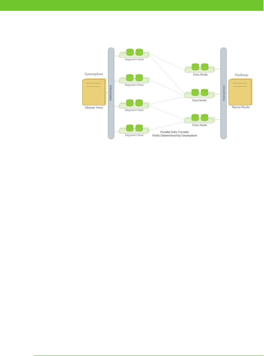
Loading Data into Greenplum Database 78

Greenplum Database DBA Guide 4.2 – Chapter 7: Loading and Unloading Data

Each Greenplum segment reads one set of Hadoop data blocks. For writing, each

Greenplum segment writes only the data contained on it.

Figure 7.1

External Table Located on a Hadoop Distributed File System

The

FORMAT

clause describes the format of the external table files. Valid file formats

are similar to the formatting options available with the PostgreSQL

COPY

command

and user-defined formats for the

gphdfs

protocol.

• Delimited text (

TEXT

) for all protocols.

• Comma separated values (

CSV

) format for

gpfdist, gpfdists,

and

file

protocols.

If the data in the file does not use the default column delimiter, escape character, null

string and so on, you must specify the additional formatting options so that Greenplum

Database reads the data in the external file correctly.

The

gphdfs

protocol requires a one-time setup. See “One-time HDFS Protocol

Installation”.

Errors in External Table Data

By default, if external table data contains an error, the command fails and no data

loads into the target database table. Define the external table with single row error

handling to enable loading correctly-formatted rows and to isolate data errors in

external table data. See “Handling Load Errors”.

The

gpfdist

file server uses the

HTTP

protocol. External table queries that use

LIMIT

end the connection after retrieving the rows, causing an

HTTP

socket error. If you use

LIMIT

in queries of external tables that use the

gpfdist://

http://

protocols,

ignore these errors – data is returned to the database as expected.

Loading Data into Greenplum Database 79

Greenplum Database DBA Guide 4.2 – Chapter 7: Loading and Unloading Data

Using the Greenplum Parallel File Server (gpfdist)

The

gpfdist

protocol provides the best performance and is the easiest to set up.

gpfdist

ensures optimum use of all segments in your Greenplum Database system

for external table reads.

This section describes the setup and management tasks for using

gpfdist

with

external tables.

• About gpfdist Setup and Performance

• Controlling Segment Parallelism

• Installing gpfdist

• Starting and Stopping gpfdist

• Troubleshooting gpfdist

About gpfdist Setup and Performance

Consider the following scenarios for optimizing your ETL network performance.

• Allow network traffic to use all ETL host Network Interface Cards (NICs)

simultaneously. Run one instance of

gpfdist

on the ETL host, then declare the

host name of each NIC in the

LOCATION

clause of your external table definition

(see “Creating External Tables - Examples” on page 93).

Figure 7.2

External Table Using Single gpfdist Instance with Multiple NICs

Loading Data into Greenplum Database 80

Greenplum Database DBA Guide 4.2 – Chapter 7: Loading and Unloading Data

• Divide external table data equally among multiple

gpfdist

instances on the ETL

host. For example, on an ETL system with two NICs, run two

gpfdist

instances

(one on each NIC) to optimize data load performance and divide the external table

data files evenly between the two

gpfdist

Figure 7.3

External Tables Using Multiple gpfdist Instances with Multiple NICs

Note: Use pipes (|) to separate formatted text when you submit files to

gpfdist

Greenplum Database encloses comma-separated text strings in single or double

quotes.

gpfdist

has to remove the quotes to parse the strings. Using pipes to

separate formatted text avoids the extra step and improves performance.

Controlling Segment Parallelism

The

gp_external_max_segs

server configuration parameter controls the number of

segment instances that can access a single

gpfdist

instance simultaneously. 64 is the

default. You can set the number of segments such that some segments process external

data files and some perform other database processing. Set this parameter in the

postgresql.conf

file of your master instance.

Installing gpfdist

gpfdist

is installed in

$GPHOME/bin

of your Greenplum Database master host

installation. Run

gpfdist

from a machine other than the Greenplum Database master,

such as on a machine devoted to ETL processing. If you want to install gpfdist on your

ETL server, get it from the Greenplum Load Tools package and follow its installation

instructions.

Starting and Stopping gpfdist

You can start gpfdist in your current directory location or in any directory that you

specify. The default port is

8080

From your current directory, type:

& gpfdist

Using Hadoop Distributed File System (HDFS) Tables 81

Greenplum Database DBA Guide 4.2 – Chapter 7: Loading and Unloading Data

From a different directory, specify the directory from which to serve files, and

optionally, the HTTP port to run on.

To start

gpfdist

in the background and log output messages and errors to a log file:

$ gpfdist -d /var/load_files -p 8081 -l /home/

gpadmin

/log &

For multiple

gpfdist

instances on the same ETL host (see Figure 7.3), use a different

base directory and port for each instance. For example:

$ gpfdist -d /var/load_files1 -p 8081 -l /home/

gpadmin

/log1 &

$ gpfdist -d /var/load_files2 -p 8082 -l /home/

gpadmin

/log2 &

To stop

gpfdist

when it is running in the background:

First find its process id:

$ ps –ef | grep gpfdist

Then kill the process, for example (where 3456 is the process ID in this example):

$ kill 3456

Troubleshooting gpfdist

The segments access

gpfdist

at runtime. Ensure that the Greenplum segment hosts

have network access to

gpfdist

is a web server: test connectivity by

running the following command from each host in the Greenplum array (segments and

master):

$ wget http://

gpfdist_hostname

port

filename

The

CREATE EXTERNAL TABLE

definition must have the correct host name, port, and

file names for

gpfdist

. Specify file names and paths relative to the directory from

which

gpfdist

serves files (the directory path specified when

gpfdist

started). See

“Creating External Tables - Examples” on page 93.

Using Hadoop Distributed File System (HDFS) Tables

Greenplum Database leverages the parallel architecture of a Hadoop Distributed File

System to read and write data files efficiently with the

gphdfs

protocol. There are

three components to using HDFS:

• One-time setup

• Grant privileges for the

HDFS

protocol

• Specify Hadoop Distributed File System data in an external table definition

One-time HDFS Protocol Installation

Install and configure Hadoop for use with

gphdfs

as follows.

1. Install Java 1.6 or later on all segments.

2. Greenplum Database includes the following Greenplum HD targets:

• The Greenplum HD target (

gphd-1.1

)

Using Hadoop Distributed File System (HDFS) Tables 82

Greenplum Database DBA Guide 4.2 – Chapter 7: Loading and Unloading Data

The default target. To use any other target, set the Server Configuration

Parameter to one of the values shown in

Table 7.1, “Server Configuration

Parameters for Hadoop Targets” on page 82.

• The Greenplum MR target for MR v. 1.0 or 1.2 (

gpmr-1.0

and

gpmr-1.2

)

If you are using

gpmr-1.0

gpmr-1.2

, install the Greenplum MR client

program. See the Setting up the Client section of the Greenplum HD MR

Administrator Guide available from Powerlink.

• The Greenplum Cloudera Hadoop Connect (

cdh3u2

3. After installation, ensure that the Greenplum system user (

gpadmin

) has read and

execute access to the Hadoop libraries or to the Greenplum MR client.

4. Set the following environment variables on all segments.

JAVA_HOME

– the Java home directory

HADOOP_HOME

– the Hadoop home directory

For example, add lines such as the following to the

gpadmin

user’s

.bashrc

profile. Note: The variables must be set in

.bashrc

because Greenplum

Database always uses SSH.

export

JAVA_HOME

=/opt/jdk1.6.0_21

export HADOOP_HOME=/bin/hadoop

5. Set the following Server Configuration Parameters.

Table 7.1

Server Configuration Parameters for Hadoop Targets

Configuration Parameter Description Default Value

Set

Classifications

gp_hadoop_target_version

The Hadoop target. Choose one

of the following.

gphd-1.1

gpmr-1.0

gpmr-1.2

cdh3u2

gphd-1.1

master

session

reload

gp_hadoop_home

Same value as

HADOOP_HOME

NULL

master

session

reload

6. Restart the database.

Grant Privileges for the HDFS Protocol

To enable privileges required to create external tables that access files on HDFS:

1. Grant the following privileges on

gphdfs

to the owner of the external table.

• Grant

SELECT

privileges to enable creating readable external tables on HDFS.

• Grant

INSERT

privileges to enable creating writable external tables on HDFS.

Use the

GRANT

command to grant read privileges (

SELECT

) and, if needed, write

privileges (

INSERT

) on HDFS to the Greenplum system user (

gpadmin

Using Hadoop Distributed File System (HDFS) Tables 83

Greenplum Database DBA Guide 4.2 – Chapter 7: Loading and Unloading Data

GRANT INSERT ON PROTOCOL gphdfs TO gpadmin;

2. Greenplum Database uses Greenplum OS credentials to connect to HDFS. Grant

read privileges and, if needed, write privileges to HDFS to the Greenplum

administrative user (

gpadmin

OS user).

Specify HDFS Data in an External Table Definition

CREATE EXTERNAL TABLE’s

LOCATION

option for Hadoop files has the following

format:

LOCATION ('gphdfs://hdfs_host[:port]/path/filename.txt')

• For any connector except

gpmr-1.0-gnet-1.0.0.1

, specify a name node port.

Do not specify a port with the

gpmr-1.0-gnet-1.0.0.1

connector.

Restrictions for

HDFS

files are as follows.

• You can specify one path for a readable external table with

gphdfs

. Wildcard

characters are allowed. If you specify a directory, the default is all files in the

directory.

You can specify only a directory for writable external tables.

• Format restrictions are as follows.

TEXT

format is allowed for readable and writable external tables.

- Only the

gphdfs_import

formatter is allowed for readable external tables

with a custom format.

- Only the

gphdfs_export

formatter is allowed for writable external tables

with a custom format.

• You can set compression only for writable external tables. Compression settings

are automatic for readable external tables.

Setting Compression Options for Hadoop Writable External Tables

Compression options for Hadoop Writable External Tables use the form of a URI

query and begin with a question mark. Specify multiple compression options with an

ampersand (

Table 7.2

Compression Options

Compression

Option

Values Default Value

compress

true

false

compress_type

BLOCK

RECORD

(Applies only to the

gphdfs_export

formatter.)

RECORD

codec Codec class name

(Applies only to the

gphdfs_export

formatter.)

GzipCodec

for text format and

DefaultCodec

for

gphdfs_expor

t format.

Place compression options in the query portion of the URI.

Using Hadoop Distributed File System (HDFS) Tables 84

Greenplum Database DBA Guide 4.2 – Chapter 7: Loading and Unloading Data

HDFS Readable and Writable External Table Examples

The following code defines a readable external table for an HDFS file named

filename.txt on port 8081.

=# CREATE EXTERNAL TABLE ext_expenses ( name text,

date date, amount float4, category text, desc1 text )

LOCATION ('gphdfs://hdfshost-1:8081/data/filename.txt')

FORMAT 'TEXT' (DELIMITER ',');

Note: Omit the port number when using the

gpmr-1.0-gnet-1.0.0.1

connector.

The following code defines a set of readable external tables that have a custom format

located in the same HDFS directory on port 8081.

=# CREATE EXTERNAL TABLE ext_expenses

LOCATION ('gphdfs://hdfshost-1:8081/data/custdat*.dat')

FORMAT 'custom' (formatter='gphdfs_import');

Note: Omit the port number when using the

gpmr-1.0-gnet-1.0.0.1

connector.

The following code defines an HDFS directory for a writable external table on port

8081 with all compression options specified.

=# CREATE WRITABLE EXTERNAL TABLE ext_expenses

LOCATION

('gphdfs://hdfshost-1:8081/data/?compress=true&compression_t

ype=BLOCK&codec=org.apache.hadoop.io.compress.DefaultCodec')

FORMAT 'custom' (formatter='gphdfs_export');

Note: Omit the port number when using the

gpmr-1.0-gnet-1.0.0.1

connector.

Because the previous code uses the default compression options for

compression_type

and

codec

, the following command is equivalent.

=# CR

EATE WRITABLE EXTERNAL TABLE ext_expenses

LOCATION ('gphdfs://hdfshost-1:8081/data?compress=true')

RMAT 'custom' (formatter='gphdfs_export');

Note: Omit the port number when using the

gpmr-1.0-gnet-1.0.0.1

connector.

Reading and Writing Custom-Formatted HDFS Data

Use MapReduce and the

CREATE EXTERNAL TABLE

command to read and write data

with custom formats on HDFS.

To read custom-formatted data:

1. Author and run a MapReduce job that creates a copy of the data in a format

accessible to Greenplum Database.

2. Use

CREATE EXTERNAL TABLE

to read the data into Greenplum Database

See “Example 1 - Read Custom-Formatted Data from HDFS” on page 85.

To write custom-formatted data:

1. Write the data.

Using Hadoop Distributed File System (HDFS) Tables 85

Greenplum Database DBA Guide 4.2 – Chapter 7: Loading and Unloading Data

2. Author and run a MapReduce program to convert the data to the custom format

and place it on the Hadoop Distributed File System.

See “Example 2 - Write Custom-Formatted Data from Greenplum Database to HDFS”

on page 87.

MapReduce is written in Java. Greenplum provides Java APIs for use in the

MapReduce code. The Javadoc is available in the

$GPHOME/docs

directory. To view

the Javadoc, expand the file gphd-xnet-1.0.0.0-javado

c.tgz

and open

index.html

The Javadoc documents the following packages:

com.emc.greenplum.gpdb.hadoop.io

com.emc.greenplum.gpdb.hadoop.mapred

com.emc.greenplum.gpdb.hadoop.mapreduce.lib.input

com.emc.greenplum.gpdb.hadoop.mapreduce.lib.output

The HDFS cross-connect packages contain the Java library, which contains the

packages

GPDBWritable

GPDBInputFormat

, and

GPDBOutputFormat

. The Java

packages are available in

$GPHOME/lib/hadoop

. For Greenplum HD, compile and

run the MapReduce job with

gphd_xnet_1.0.0.0.jar

. For Greenplum MR,

compile and run the MapReduce job with

gpmr_xnet_1.0.0.0.jar

To make the Java library available to all Hadoop users, the Hadoop cluster

administrator should place the corresponding

gphdfs

connector jar in the

$HADOOP_HOME/lib

directory and restart the job tracker. If this is not done, a Hadoop

user can still use the

gphdfs

connector jar; but with the distributed cache technique.

Example 1 - Read Custom-Formatted Data from HDFS

The sample code makes the following assumptions.

• The data is contained in HDFS directory

/demo/data/temp

and the name node is

running on port 8081.

• This code writes the data in Greenplum Database format to

/demo/data/MRTest1

on HDFS.

• The data contains the following columns, in order.

1. A long integer

2. A Boolean

3. A text string

Sample MapReduce Code

import com.emc.greenplum.gpdb.hadoop.io.GPDBWritable;

import com.emc.greenplum.gpdb.hadoop.mapreduce.lib.input.GPDBInputFormat;

import

com.emc.greenplum.gpdb.hadoop.mapreduce.lib.output.GPDBOutputFormat;

import java.io.*;

import java.util.*;

import org.apache.hadoop.fs.Path;

import org.apache.hadoop.conf.*;

import org.apache.hadoop.io.*;

import org.apache.hadoop.mapreduce.*;

import org.apache.hadoop.mapreduce.lib.output.*;

import org.apache.hadoop.mapreduce.lib.input.*;

Using Hadoop Distributed File System (HDFS) Tables 86

Greenplum Database DBA Guide 4.2 – Chapter 7: Loading and Unloading Data

import org.apache.hadoop.util.*;

public class demoMR {

* Helper routine to create our generic record. This section shows the

* format of the data. Modify as necessary.

public static GPDBWritable generateGenericRecord() throws

IOException{

int[] colType = new int[3];

colType[0] = GPDBWritable.BIGINT;

colType[1] = GPDBWritable.BOOLEAN;

colType[2] = GPDBWritable.VARCHAR;

* This section passes the values of the data. Modify as necessary.

GPDBWritable gw = new GPDBWritable(colType);

gw.setLong (0, (long)12345);

gw.setBoolean(1, true);

gw.setString (2, "abcdef");

return gw;

}

* DEMO Map/Reduce class test1

* -- Regardless of the input, this section dumps the generic record

* into GPDBFormat/

public static class Map_test1 extends Mapper<LongWritable, Text,

LongWritable, GPDBWritable> {

private LongWritable word = new LongWritable(1);

public void map(LongWritable key, Text value, Context context) throws

IOException {

try {

GPDBWritable gw = generateGenericRecord();

context.write(word, gw);

} catch (Exception e) { throw new IOException (e.getMessage()); }

}

public static void runTest1() throws Exception{

Configuration conf = new Configuration(true);

Job job = new Job(conf, "test1");

job.setJarByClass(demoMR.class);

job.setInputFormatClass(TextInputFormat.class);

job.setOutputKeyClass (LongWritable.class);

job.setOutputValueClass (GPDBWritable.class);

job.setOutputFormatClass(GPDBOutputFormat.class);

job.setMapperClass(Map_test1.class);

FileInputFormat.setInputPaths (job, new Path("/demo/data/tmp"));

Using Hadoop Distributed File System (HDFS) Tables 87

Greenplum Database DBA Guide 4.2 – Chapter 7: Loading and Unloading Data

GPDBOutputFormat.setOutputPath(job, new Path("/demo/data/MRTest1"));

job.waitForCompletion(true);

}

Run CREATE EXTERNAL TABLE

The Hadoop location corresponds to the output path in the MapReduce job.

=# CREATE EXTERNAL TABLE demodata

LOCATION ('gphdfs://hdfshost-1:8081/

demo/data/MRTest1

FORMAT 'custom' (formatter='gphdfs_import');

Note: Omit the port number when using the

gpmr-1.0-gnet-1.0.0.1

connector.

Example 2 - Write Custom-Formatted Data from Greenplum

Database to HDFS

The sample code makes the following assumptions.

• The data in Greenplum Database format is located on the Hadoop Distributed File

System on

/demo/data/writeFromGPDB_42

on port 8081.

• This code writes the data to

/demo/data/MRTest2

on port 8081.

1. Run a SQL command to create the writable table.

=# CREATE WRITABLE EXTERNAL TABLE demodata

LOCATION ('gphdfs://hdfshost-1:8081/

demo/data/MRTest2

FORMAT 'custom' (formatter='gphdfs_export');

2. Author and run code for a MapReduce job. Use the same import statements shown

“Example 1 - Read Custom-Formatted Data from HDFS” on page 85.

Note: Omit the port number when using the

gpmr-1.0-gnet-1.0.0.1

connector.

MapReduce Sample Code

* DEMO Map/Reduce class test2

* -- Convert GPDBFormat back to TEXT

public static class Map_test2 extends Mapper<LongWritable, GPDBWritable,

Text, NullWritable> {

public void map(LongWritable key, GPDBWritable value, Context context )

throws IOException {

try {

context.write(new Text(value.toString()), NullWritable.get());

} catch (Exception e) { throw new IOException (e.getMessage()); }

}

public static void runTest2() throws Exception{

Configuration conf = new Configuration(true);

Job job = new Job(conf, "test2");

job.setJarByClass(demoMR.class);

job.setInputFormatClass(GPDBInputFormat.class);

Using Hadoop Distributed File System (HDFS) Tables 88

Greenplum Database DBA Guide 4.2 – Chapter 7: Loading and Unloading Data

job.setOutputKeyClass (Text.class);

job.setOutputValueClass(NullWritable.class);

job.setOutputFormatClass(TextOutputFormat.class);

job.setMapperClass(Map_test2.class);

GPDBInputFormat.setInputPaths (job,

new Path("/demo/data/writeFromGPDB_42"));

GPDBOutputFormat.setOutputPath(job, new Path("/demo/data/MRTest2"));

job.waitForCompletion(true);

}

Creating and Using Web External Tables

CREATE EXTERNAL WEB TABLE

creates a web table definition. Web external tables

allow Greenplum Database to treat dynamic data sources like regular database tables.

Because web table data can change as a query runs, the data is not rescannable.

You can define command-based or URL-based web external tables. The definition

forms are distinct: you cannot mix command-based and URL-based definitions.

Command-based Web External Tables

The output of a shell command or script defines command-based web table data.

Specify the command in the

EXECUTE

clause of

CREATE EXTERNAL WEB TABLE.

The

data is current as of the time the command runs. The

EXECUTE

clause runs the shell

command or script on the specified master, and/or segment host or hosts. The

command or script must reside on the hosts corresponding to the host(s) defined in the

EXECUTE

clause.

By default, all active segments run the command on all segment hosts. For example, if

each segment host runs four primary segment instances, the command runs four times

per segment host. You can optionally limit the number of segment instances that

execute the web table command. All segments included in the web table definition in

the

clause run the command in parallel.

The command that you specify in the external table definition executes from the

database and cannot access environment variables from

.bashrc

.profile

. Set

environment variables in the

EXECUTE

clause. For example:

=# CREATE EXTERNAL WEB TABLE output (output text)

EXECUTE 'PATH=/home/

gpadmin

/programs; export PATH;

myprogram.sh'

FORMAT 'TEXT';

Scripts must be executable by the

gpadmin

user and reside in the same location on the

master or segment hosts.

The following command defines a web table that runs a script once on each segment

host.

=# CREATE EXTERNAL WEB TABLE log_output

(linenum int, message text)

EXECUTE '/var/load_scripts/get_log_data.sh' ON HOST

Using Hadoop Distributed File System (HDFS) Tables 89

Greenplum Database DBA Guide 4.2 – Chapter 7: Loading and Unloading Data

FORMAT 'TEXT' (DELIMITER '|');

URL-based Web External Tables

A URL-based web table accesses data from a web server using the HTTP protocol.

Web table data is dynamic: the data is not rescannable.

Specify the

LOCATION

of files on a web server using

http://

. The web data file(s)

must reside on a web server that Greenplum segment hosts can access. The number of

URLs specified corresponds to the number of segment instances that work in parallel

to access the web table. For example, if you specify 2 external files to a Greenplum

Database system with 8 primary segments, 2 of the 8 segments access the web table in

parallel at query runtime.

The following sample command defines a web table that gets data from several URLs.

=# CREATE EXTERNAL WEB TABLE ext_expenses (name text,

date date, amount float4, category text, description text)

LOCATION (

'http://intranet.company.com/expenses/sales/file.csv',

'http://intranet.company.com/expenses/exec/file.csv',

'http://intranet.company.com/expenses/finance/file.csv',

'http://intranet.company.com/expenses/ops/file.csv',

'http://intranet.company.com/expenses/marketing/file.csv',

'http://intranet.company.com/expenses/eng/file.csv'

)

FORMAT 'CSV' ( HEADER );

Loading Data Using an External Table

Use SQL commands such as

INSERT

and

SELECT

to query a readable external table,

the same way that you query a regular database table. For example, to load travel

expense data from an external table, ext_expenses, into a database table,

expenses_travel:

=# INSERT INTO expenses_travel

SELECT * from ext_expenses where category='travel';

To load all data into a new database table:

=# CREATE TABLE expenses AS SELECT * from ext_expenses;

Loading and Writing Non-HDFS Custom Data

Greenplum supports

TEXT

and

CSV

formats for importing and exporting data. You can

load and write the data in other formats by defining and using a custom format or

custom protocol.

• Using a Custom Format

• Using a Custom Protocol

For information about importing custom data from HDFS, see “Reading and Writing

Custom-Formatted HDFS Data” on page 84.

Using Hadoop Distributed File System (HDFS) Tables 90

Greenplum Database DBA Guide 4.2 – Chapter 7: Loading and Unloading Data

Using a Custom Format

You specify a custom data format in the

FORMAT

clause of

CREATE EXTERNAL TABLE

FORMAT ‘CUSTOM’ (formatter=format_function,

key1=val1,...keyn=valn)

Where the ‘

CUSTOM

’ keyword indicates that the data has a custom format and

formatter

specifies the function to use to format the data, followed by

comma-separated parameters to the formatter function.

Greenplum Database provides functions for formatting fixed-width data, but you must

author the formatter functions for variable-width data. The steps are as follows.

1. Author and compile input and output functions as a shared library.

2. Specify the shared library function with

CREATE FUNCTION

in Greenplum

Database.

3. Use the

formatter

parameter of

CREATE EXTERNAL TABLE’s FORMAT

clause

to call the function.

Importing and Exporting Fixed Width Data

Specify custom formats for fixed-width data with the Greenplum Database

functions

fixedwith_in

and

fixedwidth_out

. These functions already exist in the file

$GPHOME\share\postgresql\cdb_external_extensions.sql. The following example

declares a custom format, then calls the

fixedwidth_in

function to format the data.

CREATE READABLE EXTERNAL TABLE students (

name varchar(20), address varchar(30), age int)

LOCATION ('file://<host>/file/path/')

FORMAT 'CUSTOM' (formatter=fixedwidth_in,

name='20', address='30', age='4');

The following options specify how to import fixed width data.

• Read all the data.

To load all the fields on a line of fixed with data, you must load them in their

physical order. You must specify the field length, but cannot specify a starting and

ending position. The fields names in the fixed width arguments must match the

order in the field list at the beginning of the

CREATE TABLE

command.

• Set options for blank and null characters.

Trailing blanks are trimmed by default. To keep trailing blanks, use the

preserve_blanks=on

option.You can reset the trailing blanks option to the

default with the

preserve_blanks=off

option.

Use the null=

'null_string_value'

option to specify a value for null

characters.

- If you specify

preserve_blanks=on

, you must also define a value for null

characters.

- If you specify

preserve_blanks=off

, null is not defined, and the field

contains only blanks, Greenplum writes a null to the table. If null is defined,

Greenplum writes an empty string to the table.

Using Hadoop Distributed File System (HDFS) Tables 91

Greenplum Database DBA Guide 4.2 – Chapter 7: Loading and Unloading Data

Use the

line_delim='line_ending'

parameter to specify the line ending

character. The following examples cover most cases. The E specifies an escape

string constant.

line_delim=E'\n'

line_delim=E'\r'

line_delim=E'\r\n'

line_delim='abc'

Examples: Read Fixed-Width Data

The following examples show how to read fixed-width data.

Example 1 – Loading a table with all fields defined

CREATE READABLE EXTERNAL TABLE students (

name varchar(20), address varchar(30), age int)

LOCATION ('file://<host>/file/path/')

FORMAT 'CUSTOM' (formatter=fixedwidth_in,

name=20, address=30, age=4);

Example 2 – Loading a table with PRESERVED_BLANKS ON

CREATE READABLE EXTERNAL TABLE students (

name varchar(20), address varchar(30), age int)

LOCATION ('gpfdist://<host>:<portNum>/file/path/')

FORMAT 'CUSTOM' (formatter=fixedwidth_in,

name=20, address=30, age=4,

preserve_blanks='on',null='NULL');

Example 3 – Loading data with no line delimiter

CREATE READABLE EXTERNAL TABLE students (

name varchar(20), address varchar(30), age int)

LOCATION ('file://<host>/file/path/')

FORMAT 'CUSTOM' (formatter=fixedwidth_in,

name='20', address='30', age='4', line_delim='?@')

Example 4 – Create a writable external table with a \r\n line delimiter

CREATE WRITABLE EXTERNAL TABLE students_out (

name varchar(20), address varchar(30), age int)

LOCATION ('gpfdist://<host>:<portNum>/file/path/')

FORMAT 'CUSTOM' (formatter=fixedwidth_out,

name=20, address=30, age=4, line_delim=E'\r\n');

Using a Custom Protocol

Greenplum provides protocols such as

gpfdist

http

, and

file

for accessing data

over a network, or you can author a custom protocol. You can use the standard data

formats,

TEXT

and

CSV

, or a custom data format with custom protocols.

Using Hadoop Distributed File System (HDFS) Tables 92

Greenplum Database DBA Guide 4.2 – Chapter 7: Loading and Unloading Data

Declare custom protocols with the SQL command

CREATE TRUSTED PROTOCOL,

then

use the

GRANT

command to grant access to your users. For example:

• Allow a user to create a readable external table with a trusted protocol

GRANT SELECT ON PROTOCOL <protocol name> TO <user name>

• Allow a user to create a writable external table with a trusted protocol

GRANT INSERT ON PROTOCOL <protocol name> TO <user name>

• Allow a user to create readable and writable external tables with a trusted protocol

GRANT ALL ON PROTOCOL <protocol name> TO <user name>

The following steps describe authoring and using a custom protocol.

1. Author the send, receive, and (optionally) validator functions in C, with a

predefined API. These functions are compiled and registered with the Greenplum

Database.

The following examples use the compiled import and export code.

CREATE FUNCTION myread() RETURNS integer

as '$libdir/gpextprotocol.so', 'myprot_import'

LANGUAGE C STABLE;

CREATE FUNCTION mywrite() RETURNS integer

as '$libdir/gpextprotocol.so', 'myprot_export'

LANGUAGE C STABLE;

The format of the optional function is:

CREATE OR REPLACE FUNCTION myvalidate() RETURNS void

AS '$libdir/gpextprotocol.so', 'myprot_validate'

LANGUAGE C STABLE;

2. Create a protocol that accesses these functions.

Validatorfunc

is optional.

CREATE TRUSTED PROTOCOL myprot(

writefunc='mywrite'

readfunc='myread',

validatorfunc='myvalidate');

3. Grant access to any other users, as necessary

GRANT ALL ON PROTOCOL myprot TO otheruser

4. Use the protocol in readable or writable external tables.

CREATE WRITABLE EXTERNAL TABLE ext_sales(LIKE sales)

LOCATION ('myprot://<meta>/<meta>/…')

FORMAT 'TEXT';

CREATE READABLE EXTERNAL TABLE ext_sales(LIKE sales)

LOCATION('myprot://<meta>/<meta>/…')

FORMAT 'TEXT';

Using Hadoop Distributed File System (HDFS) Tables 93

Greenplum Database DBA Guide 4.2 – Chapter 7: Loading and Unloading Data

Creating External Tables - Examples

The following examples show how to define external data with different protocols.

Each

CREATE EXTERNAL TABLE

command can contain only one protocol.

Note: When using IPv6, always enclose the numeric IP addresses in square brackets.

Start

gpfdist

before you create external tables with the

gpfdist

protocol. The

following code starts the

gpfdist

file server program in the background on port 8081

serving files from directory /var/data/staging. The logs are saved in

/home/gpadmin/log.

gpfdist -p 8081 -d /var/data/staging -l /home/

gpadmin

/log &

The

CREATE EXTERNAL TABLE

SQL command defines external tables, the location

and format of the data to load, and the protocol to use to load the data, but does not

load data into the table. For example, the following command creates an external

table,

ext_expenses

, from pipe (‘|’) delimited text data located on

etlhost-1:8081 and etlhost-2:8081. See the Greenplum Database

Reference Guide for information about

CREATE EXTERNAL TABLE.

Example 1—Single gpfdist instance on single-NIC machine

Creates a readable external table, ext_expenses, using the

gpfdist

protocol. The files

are formatted with a pipe ( | ) as the column delimiter.

=# CREATE EXTERNAL TABLE ext_expenses ( name text,

date date, amount float4, category text, desc1 text )

LOCATION ('gpfdist://etlhost-1:8081/*',

'gpfdist://etlhost-1:8082/*')

FORMAT 'TEXT' (DELIMITER '|');

Example 2—Multiple gpfdist instances

Creates a readable external table, ext_expenses, using the

gpfdist

protocol from all

files with the txt extension. The column delimiter is a pipe ( | ) and NULL (‘ ‘) is a

space.

=# CREATE EXTERNAL TABLE ext_expenses ( name text,

date date, amount float4, category text, desc1 text )

LOCATION ('gpfdist://etlhost-1:8081/*.txt',

'gpfdist://etlhost-2:8081/*.txt')

FORMAT 'TEXT' ( DELIMITER '|' NULL ' ') ;

Example 3—Multiple gpfdists instances

Creates a readable external table, ext_expenses, from all files with the txt extension

using the

gpfdists

protocol. The column delimiter is a pipe ( | ) and NULL (‘ ‘) is a

space. For information about the location of security certificates, see

“gpfdists” on

page 76.

1. Run gpfdist with the

--ssl

option.

2. Run the following command.

=# CREATE EXTERNAL TABLE ext_expenses ( name text,

Using Hadoop Distributed File System (HDFS) Tables 94

Greenplum Database DBA Guide 4.2 – Chapter 7: Loading and Unloading Data

date date, amount float4, category text, desc1 text )

LOCATION ('gpfdists://etlhost-1:8081/*.txt',

'gpfdists://etlhost-2:8082/*.txt')

FORMAT 'TEXT' ( DELIMITER '|' NULL ' ') ;

Example 4—Single gpfdist instance with error logging

Uses the gpfdist protocol to create a readable external table, ext_expenses, from all

files with the txt extension. The column delimiter is a pipe ( | ) and NULL (‘ ‘) is a

space.

Access to the external table is single row error isolation mode. Input data formatting

errors are written to the error table,

err_customer,

with a description of the error.

Query

err_customer

to see the errors, then fix the issues and reload the rejected data.

If the error count on a segment is greater than five (the

SEGMENT REJECT LIMIT

value), the entire external table operation failes and no rows are processed.

=# CREATE EXTERNAL TABLE ext_expenses ( name text,

date date, amount float4, category text, desc1 text )

LOCATION ('gpfdist://etlhost-1:8081/*.txt',

'gpfdist://etlhost-2:8082/*.txt')

FORMAT 'TEXT' ( DELIMITER '|' NULL ' ')

LOG ERRORS INTO err_customer SEGMENT REJECT LIMIT 5;

To create the readable ext_expenses table from CSV-formatted text files:

=# CREATE EXTERNAL TABLE ext_expenses ( name text,

date date, amount float4, category text, desc1 text )

LOCATION ('gpfdist://etlhost-1:8081/*.txt',

'gpfdist://etlhost-2:8082/*.txt')

FORMAT 'CSV' ( DELIMITER ',' )

LOG ERRORS INTO err_customer SEGMENT REJECT LIMIT 5;

Example 5—TEXT Format on a Hadoop Distributed File Server

Creates a readable external table, ext_expenses, using the

gphdfs

protocol. The

column delimiter is a pipe ( | ).

=# CREATE EXTERNAL TABLE ext_expenses ( name text,

date date, amount float4, category text, desc1 text )

LOCATION ('gphdfs://hdfshost-1:8081/data/filename.txt')

FORMAT 'TEXT' (DELIMITER '|');

Note: gphdfs requires only one data path.

For examples of reading and writing custom formatted data on a Hadoop Distributed

File System, see

“Reading and Writing Custom-Formatted HDFS Data” on page 84.

Example 6—Multiple files in CSV format with header rows

Creates a readable external table, ext_expenses, using the

file

protocol. The files are

CSV

format and have a header row.

=# CREATE EXTERNAL TABLE ext_expenses ( name text,

Using Hadoop Distributed File System (HDFS) Tables 95

Greenplum Database DBA Guide 4.2 – Chapter 7: Loading and Unloading Data

date date, amount float4, category text, desc1 text )

LOCATION ('file://filehost:5432/data/international/*',

'file://filehost:5432/data/regional/*'

'file://filehost:5432/data/supplement/*.csv')

FORMAT 'CSV' (HEADER);

Example 7—Readable Web External Table with Script

Creates a readable web external table that executes a script once per segment host:

=# CREATE EXTERNAL WEB TABLE log_output (linenum int,

message text)

EXECUTE '/var/load_scripts/get_log_data.sh' ON HOST

FORMAT 'TEXT' (DELIMITER '|');

Example 8—Writable External Table with gpfdist

Creates a writable external table, sales_out, that uses

gpfdist

to write output data to

the file sales.out. The column delimiter is a pipe ( | ) and NULL (‘ ‘) is a space. The

file will be created in the directory specified when you started the gpfdist file server.

=# CREATE WRITABLE EXTERNAL TABLE sales_out (LIKE sales)

LOCATION ('gpfdist://etl1:8081/sales.out')

FORMAT 'TEXT' ( DELIMITER '|' NULL ' ')

DISTRIBUTED BY (txn_id);

Example 9—Writable External Web Table with Script

Creates a writable external web table, campaign_out, that pipes output data received

by the segments to an executable script, to_adreport_etl.sh:

=# CREATE WRITABLE EXTERNAL WEB TABLE campaign_out

(LIKE campaign)

EXECUTE '/var/unload_scripts/to_adreport_etl.sh'

FORMAT 'TEXT' (DELIMITER '|');

Example 10—Readable and Writable External Tables with XML

Transformations

Greenplum Database can read and write XML data to and from external tables with

gpfdist. For information about setting up an XML transform, see

“Transforming XML

Data” on page 104.

Handling Load Errors

Readable external tables are most commonly used to select data to load into regular

database tables. You use the

CREATE TABLE AS SELECT

INSERT INTO

commands

to query the external table data. By default, if the data contains an error, the entire

command fails and the data is not loaded into the target database table.

The

SEGMENT REJECT LIMIT

clause allows you to isolate format errors in external

table data and to continue loading correctly formatted rows. Use

SEGMENT REJECT

LIMIT

to set an error threshold, specifying the reject limit

count

as number of

ROWS

(the default) or as a

PERCENT

of total rows (1-100).

Using Hadoop Distributed File System (HDFS) Tables 96

Greenplum Database DBA Guide 4.2 – Chapter 7: Loading and Unloading Data

The entire external table operation is aborted, and no rows are processed, if the

number of error rows reaches the

SEGMENT REJECT LIMIT

. The limit of error rows is

per-segment, not per entire operation. The operation processes all good rows, and it

discards or logs any erroneous rows into an error table (if you specified an error table),

if the number of error rows does not reach the

SEGMENT REJECT LIMIT

The

LOG ERRORS INTO

clause allows you to keep error rows for further examination.

Use

LOG ERRORS INTO

to declare

an error table in which to write error rows.

When you set

SEGMENT REJECT LIMIT

, Greenplum scans the external data in single

row error isolation mode. Single row error isolation mode applies to external data

rows with format errors such as extra or missing attributes, attributes of a wrong data

type, or invalid client encoding sequences. Greenplum does not check constraint

errors, but you can filter constraint errors by limiting the

SELECT

from an external

table at runtime. For example, to eliminate duplicate key errors:

=# INSERT INTO table_with_pkeys

SELECT DISTINCT * FROM external_table;

Define an External Table with Single Row Error Isolation

The following example creates an external table, ext_expenses, sets an error threshold

of 10 errors, and writes error rows to the table err_expenses.

=# CREATE EXTERNAL TABLE ext_expenses ( name text,

date date, amount float4, category text, desc1 text )

LOCATION ('gpfdist://etlhost-1:8081/*',

'gpfdist://etlhost-2:8082/*')

FORMAT 'TEXT' (DELIMITER '|')

LOG ERRORS INTO err_expenses SEGMENT REJECT LIMIT 10

ROWS;

Create an Error Table and Declare a Reject Limit

The following SQL fragment creates an error table, err_expenses, and declares a reject

limit of 10 rows.

LOG ERRORS INTO err_expenses SEGMENT REJECT LIMIT 10 ROWS

Viewing Bad Rows in the Error Table

If you use single row error isolation (see “Define an External Table with Single Row

Error Isolation” on page 96 or “Running COPY in Single Row Error Isolation Mode”

on page 99), any rows with formatting errors are logged into an error table. The error

table has the following columns:

Table 7.3

Error Table Format

column type description

cmdtime timestampz Timestamp when the error occurred.

relname text The name of the external table or the

target table of a COPY command.

filename text The name of the load file that

contains the error.

Using Hadoop Distributed File System (HDFS) Tables 97

Greenplum Database DBA Guide 4.2 – Chapter 7: Loading and Unloading Data

You can use SQL commands to query the error table and view the rows that did not

load. For example:

=# SELECT * from err_expenses;

Identifying Invalid CSV Files in Error Table Data

If a CSV file contains invalid formatting, the rawdata field in the error table can

contain several combined rows. For example, if a closing quote for a specific field is

missing, all the following newlines are treated as embedded newlines. When this

happens, Greenplum stops parsing a row when it reaches 64K, puts that 64K of data

into the error table as a single row, resets the quote flag, and continues. If this happens

three times during load processing, the load file is considered invalid and the entire

load fails with the message “

rejected

or more rows

”. See “Escaping in CSV

Formatted Files” on page 117 for more information on the correct use of quotes in

CSV files.

Moving Data between Tables

You can use

CREATE TABLE AS

INSERT...SELECT

to load external and web

external table data into another (non-external) database table, and the data will be

loaded in parallel according to the external or web external table definition.

If an external table file or web external table data source has an error, one of the

following will happen, depending on the isolation mode used:

linenum int If COPY was used, the line number

in the load file where the error

occurred. For external tables using

file:// protocol or gpfdist:// protocol

and CSV format, the file name and

line number is logged.

bytenum int For external tables with the gpfdist://

protocol and data in TEXT format:

the byte offset in the load file where

the error occurred. gpfdist parses

TEXT files in blocks, so logging a line

number is not possible.

CSV files are parsed a line at a time

so line number tracking is possible

for CSV files.

errmsg text The error message text.

rawdata text The raw data of the rejected row.

rawbytes bytea In cases where there is a database

encoding error (the client encoding

used cannot be converted to a

server-side encoding), it is not

possible to log the encoding error as

rawdata. Instead the raw bytes are

stored and you will see the octal

code for any non seven bit ASCII

characters.

Table 7.3

Error Table Format

column type description

Using Hadoop Distributed File System (HDFS) Tables 98

Greenplum Database DBA Guide 4.2 – Chapter 7: Loading and Unloading Data

• Tables without error isolation mode: any operation that reads from that table

fails. Loading from external and web external tables without error isolation mode

is an all or nothing operation.

• Tables with error isolation mode: the entire file will be loaded, except for the

problematic rows (subject to the configured REJECT_LIMIT)

Loading Data

The following methods load data from readable external tables.

• Use the

gpload

utility

• Use the

gphdfs

protocol

• Load with

copy

Loading Data with gpload

The Greenplum

gpload

utility loads data using readable external tables and the

Greenplum parallel file server (

gpfdist

gpfdists

). It handles parallel file-based

external table setup and allows users to configure their data format, external table

definition, and

gpfdist

gpfdists

setup in a single configuration file.

To use gpload

1. Ensure that your environment is set up to run

gpload

. Some dependent files from

your Greenplum Database installation are required, such as

gpfdist

and Python,

as well as network access to the Greenplum segment hosts. See the Greenplum

Database Reference Guide for details.

2. Create your load control file. This is a YAML-formatted file that specifies the

Greenplum Database connection information,

gpfdist

configuration

information, external table options, and data format. See the Greenplum Database

Reference Guide for details.

For example:

---

VERSION: 1.0.0.1

DATABASE: ops

USER: gpadmin

HOST: mdw-1

PORT: 5432

GPLOAD:

INPUT:

- SOURCE:

LOCAL_HOSTNAME:

- etl1-1

- etl1-2

- etl1-3

- etl1-4

PORT: 8081

FILE:

- /var/load/data/*

Using Hadoop Distributed File System (HDFS) Tables 99

Greenplum Database DBA Guide 4.2 – Chapter 7: Loading and Unloading Data

- COLUMNS:

- name: text

- amount: float4

- category: text

- desc: text

- date: date

- FORMAT: text

- DELIMITER: '|'

- ERROR_LIMIT: 25

- ERROR_TABLE: payables.err_expenses

OUTPUT:

- TABLE: payables.expenses

- MODE: INSERT

SQL:

- BEFORE: "INSERT INTO audit VALUES('start', current_timestamp)"

- AFTER: "INSERT INTO audit VALUES('end', current_timestamp)"

3. Run

gpload

, passing in the load control file. For example:

gpload -f my_load.yml

Loading Data with the gphdfs Protocol

If you use

INSERT INTO

to insert data into a Greenplum table from a table on the

Hadoop Distributed File System that was defined as an external table with the gphdfs

protocol, the data is copied in parallel. For example:

INSERT INTO

gpdb_table (select * from hdfs_ext_table);

Loading Data with COPY

COPY

FROM

copies data from a file or standard input into a table and appends the data

to the table contents.

COPY

is non-parallel: data is loaded in a single process using the

Greenplum master instance.

To optimize the performance and throughput of

COPY

, run multiple

COPY

commands

concurrently in separate sessions and divide the data evenly across all concurrent

processes. To optimize throughput, run one concurrent

COPY

operation per CPU.

The

COPY

source file must be accessible to the master host. Specify the

COPY

source

file name relative to the master host location.

Greenplum copies data from

STDIN

STDOUT

using the connection between the

client and the master server.

Running COPY in Single Row Error Isolation Mode

By default,

COPY

stops an operation at the first error: if the data contains an error, the

operation fails and no data loads. If you run

COPY FROM

in single row error isolation

mode, Greenplum skips rows that contain format errors and loads properly formatted

rows. Single row error isolation mode applies only to rows in the input file that

contain format errors. If the data contains a contraint error such as violation of a

NOT

NULL

CHECK

, or

UNIQUE

constraint, the operation fails and no data loads.

Unloading Data from Greenplum Database 100

Greenplum Database DBA Guide 4.2 – Chapter 7: Loading and Unloading Data

Specifying

SEGMENT REJECT LIMIT

runs the

COPY

operation in single row error

isolation mode. Specify the acceptable number of error rows on each segment, after

which the entire

COPY FROM

operation fails and no rows load. The error row count is

for each Greenplum segment, not for the entire load operation.

If the

COPY

operation does not reach the error limit, Greenplum loads all

correctly-formatted rows and discards the error rows. The

LOG ERRORS INTO

clause

allows you to keep error rows for further examination. Use

LOG ERRORS INTO

declare

an error table in which to write error rows. For example:

=> COPY country FROM '/data/gpdb/country_data'

WITH DELIMITER '|' LOG ERRORS INTO err_country

SEGMENT REJECT LIMIT 10 ROWS;

See “Viewing Bad Rows in the Error Table” on page 96 for information about

investigating error rows.

Optimizing Data Load and Query Performance

Use the following tips to help optimize your data load and subsequent query

performance.

• Drop indexes before loading data into existing tables.

Creating an index on pre-existing data is faster than updating it incrementally as

each row is loaded. You can temporarily increase the maintenance_work_mem

server configuration parameter to help speed up

CREATE INDEX

commands,

though load performance is affected. Drop and recreate indexes only when there

are no active users on the system.

• Create indexes last when loading data into new tables. Create the table, load the

data, and create any required indexes.

• Run

ANALYZE

after loading data. If you significantly altered the data in a table, run

ANALYZE

VACUUM ANALYZE

to update table statistics for the query planner.

Current statistics ensure that the planner makes the best decisions during query

planning and avoids poor performance due to inaccurate or nonexistent statistics.

• Run

VACUUM

after load errors. If the load operation does not run in single row error

isolation mode, the operation stops at the first error. The target table contains the

rows loaded before the error occurred. You cannot access these rows, but they

occupy disk space. Use the

VACUUM

command to recover the wasted space.

Unloading Data from Greenplum Database

A writable external table allows you to select rows from other database tables and

output the rows to files, named pipes, to applications, or as output targets for

Greenplum parallel MapReduce calculations. You can define file-based and

web-based writable external tables.

This section describes how to unload data from Greenplum Database using parallel

unload (writable external tables) and non-parallel unload (

COPY

• Defining a File-Based Writable External Table

• Defining a Command-Based Writable External Web Table

Unloading Data from Greenplum Database 101

Greenplum Database DBA Guide 4.2 – Chapter 7: Loading and Unloading Data

• Unloading Data Using a Writable External Table

• Unloading Data Using COPY

Defining a File-Based Writable External Table

Writable external tables that output data to files use the Greenplum parallel file server

program,

gpfdist

, or the Hadoop Distributed File System interface,

gphdfs

Use the

CREATE WRITABLE EXTERNAL TABLE

command to define the external table

and specify the location and format of the output files. See

“Using the Greenplum

Parallel File Server (gpfdist)” on page 79 for instructions on setting up

gpfdist

for

use with an external table and “Using Hadoop Distributed File System (HDFS)

Tables” on page 81 for instructions on setting up

gphdfs

for use with an external

table.

• With a writable external table using the

gpfdist

protocol, the Greenplum

segments send their data to

gpfdist

, which writes the data to the named file.

gpfdist

must run on a host that the Greenplum segments can access over the

network.

gpfdist

points to a file location on the output host and writes data

received from the Greenplum segments to the file. To divide the output data

among multiple files, list multiple

gpfdist

URIs in your writable external table

definition.

• A writable external web table sends data to an application as a stream of data. For

example, unload data from Greenplum Database and send it to an application that

connects to another database or ETL tool to load the data elsewhere. Writable

external web tables use the

EXECUTE

clause to specify a shell command, script, or

application to run on the segment hosts and accept an input stream of data. See

“Defining a Command-Based Writable External Web Table” for more

information about using

EXECUTE

commands in a writable external table

definition.

You can optionally declare a distribution policy for your writable external tables. By

default, writable external tables use a random distribution policy. If the source table

you are exporting data from has a hash distribution policy, defining the same

distribution key column(s) for the writable external table improves unload

performance by eliminating the requirement to move rows over the interconnect. If

you unload data from a particular table, you can use the

clause to copy the

column definitions and distribution policy from the source table.

Example 1—Greenplum file server (gpfdist)

=# CREATE WRITABLE EXTERNAL TABLE unload_expenses

( LIKE expenses )

LOCATION ('gpfdist://etlhost-1:8081/expenses1.out',

'gpfdist://etlhost-2:8081/expenses2.out')

FORMAT 'TEXT' (DELIMITER ',')

DISTRIBUTED BY (exp_id);

Example 2—Hadoop file server (gphdfs)

=# CREATE WRITABLE EXTERNAL TABLE unload_expenses

Unloading Data from Greenplum Database 102

Greenplum Database DBA Guide 4.2 – Chapter 7: Loading and Unloading Data

( LIKE expenses )

LOCATION ('gphdfs://hdfslhost-1:8081/path')

FORMAT 'TEXT' (DELIMITER ',')

DISTRIBUTED BY (exp_id);

You can only specify a directory for a writable external table with the

gphdfs

protocol. (You can only specify one file for a readable external table with the

gphdfs

protocol)

Note: The default port number is 9000.

Defining a Command-Based Writable External Web Table

You can define writable external web tables to send output rows to an application or

script. The application must accept an input stream, reside in the same location on all

of the Greenplum segment hosts, and be executable by the

gpadmin

user. All

segments in the Greenplum system run the application or script, whether or not a

segment has output rows to process.

Use

CREATE WRITABLE EXTERNAL WEB TABLE

to define the external table and

specify the application or script to run on the segment hosts. Commands execute from

within the database and cannot access environment variables (such as

$PATH

). Set

environment variables in the

EXECUTE

clause of your writable external table

definition. For example:

=# CREATE WRITABLE EXTERNAL WEB TABLE output (output text)

EXECUTE 'export PATH=$PATH:/home/

gpadmin

/programs;

myprogram.sh'

FORMAT 'TEXT'

DISTRIBUTED RANDOMLY;

The following Greenplum Database variables are available for use in OS commands

executed by a web or writable external table. Set these variables as environment

variables in the shell that executes the command(s). They can be used to identify a set

of requests made by an external table statement across the Greenplum Database array

of hosts and segment instances.

Table 7.4

External Table EXECUTE Variables

Variable Description

$GP_CID Command count of the session executing the external table

statement.

$GP_DATABASE The database in which the external table definition resides.

$GP_DATE The date on which the external table command ran.

$GP_MASTER_HOST The host name of the Greenplum master host from which the external

table statement was dispatched.

$GP_MASTER_PORT The port number of the Greenplum master instance from which the

external table statement was dispatched.

$GP_SEG_DATADIR The location of the data directory of the segment instance executing

the external table command.

Unloading Data from Greenplum Database 103

Greenplum Database DBA Guide 4.2 – Chapter 7: Loading and Unloading Data

Disabling EXECUTE for Web or Writable External Tables

There is a security risk associated with allowing external tables to execute OS

commands or scripts. To disable the use of

EXECUTE

in web and writable external table

definitions, set the

gp_external_enable_exec server configuration parameter to

off in your master

postgresql.conf

file:

gp_external_enable_exec = off

Unloading Data Using a Writable External Table

Writable external tables allow only

INSERT

operations. You must grant

INSERT

permission on a table to enable access to users who are not the table owner or a

superuser. For example:

GRANT INSERT ON writable_ext_table TO admin;

To unload data using a writable external table, select the data from the source table(s)

and insert it into the writable external table. The resulting rows are output to the

writable external table. For example:

INSERT INTO writable_ext_table SELECT * FROM regular_table;

Unloading Data Using COPY

COPY

copies data from a table to a file (or standard input) on the Greenplum master

host using a single process on the Greenplum master instance. Use

COPY

to output a

table’s entire contents, or filter the output using a

SELECT

statement. For example:

COPY (SELECT * FROM country WHERE country_name LIKE 'A%') TO

'/home/

gpadmin

/a_list_countries.out';

$GP_SEG_PG_CONF

The location of the

postgresql.conf

file of the segment instance

executing the external table command.

$GP_SEG_PORT The port number of the segment instance executing the external table

command.

$GP_SEGMENT_COUNT The total number of primary segment instances in the Greenplum

Database system.

$GP_SEGMENT_ID The ID number of the segment instance executing the external table

command (same as

dbid

gp_segment_configuration

$GP_SESSION_ID The database session identifier number associated with the external

table statement.

$GP_SN Serial number of the external table scan node in the query plan of the

external table statement.

$GP_TIME The time the external table command was executed.

$GP_USER The database user executing the external table statement.

$GP_XID The transaction ID of the external table statement.

Table 7.4

External Table EXECUTE Variables

Variable Description

Transforming XML Data 104

Greenplum Database DBA Guide 4.2 – Chapter 7: Loading and Unloading Data

Transforming XML Data

The Greenplum Database data loader gpfdist provides transformation features to load

XML data into a table and to write data from the Greenplum Database to XML files.

The following diagram shows gpfdist performing an XML transform.

Figure 7.4

External Tables using XML Transformations

To load or extract XML data:

• Determine the Transformation Schema

• Write a Transform

• Write the gpfdist Configuration

• Load the Data

• Transfer and Store the Data

The first three steps comprise most of the development effort. The last two steps are

straightforward and repeatable, suitable for production.

Determine the Transformation Schema

To prepare for the transformation project:

1. Determine the goal of the project, such as indexing data, analyzing data,

combining data, and so on.

2. Examine the XML file and note the file structure and element names.

3. Choose the elements to import and decide if any other limits are appropriate.

For example, the following XML file, prices.xml, is a simple, short file that contains

price records. Each price record contains two fields: an item number and a price.

Transforming XML Data 105

Greenplum Database DBA Guide 4.2 – Chapter 7: Loading and Unloading Data

<?xml version="1.0" encoding="ISO-8859-1" ?>

</pricerecord>

</pricerecord>

</pricerecord>

</prices>

The goal is to import all the data into a Greenplum Database table with an integer

itemnumber

column and a decimal

price

column.

Write a Transform

The transform specifies what to extract from the data.You can use any authoring

environment and language appropriate for your project. For XML transformations

Greenplum suggests choosing a technology such as XSLT, Joost (STX), Java, Python,

or Perl, based on the goals and scope of the project.

In the price example, the next step is to transform the XML data into a simple

two-column delimited format.

708421|19.99

708466|59.25

711121|24.99

The following STX transform, called input_transform.stx, completes the data

transformation.

<?xml version="1.0"?>

<stx:transform version="1.0"

xmlns:stx="http://stx.sourceforge.net/2002/ns"

pass-through="none">

<stx:variable name="itemnumber"/>

<stx:variable name="price"/>

<stx:template match="/prices/pricerecord">

<stx:process-children/>

<stx:value-of select="$itemnumber"/>

<stx:text>|</stx:text>

<stx:value-of select="$price"/> <stx:text>

</stx:text>

</stx:template>

Transforming XML Data 106

Greenplum Database DBA Guide 4.2 – Chapter 7: Loading and Unloading Data

<stx:template match="itemnumber">

<stx:assign name="itemnumber" select="."/>

</stx:template>

<stx:template match="price">

<stx:assign name="price" select="."/>

</stx:template>

</stx:transform>

This STX transform declares two temporary variables,

itemnumber

and

price

, and

the following rules.

1. When an element that satisfies the XPath expression

/prices/pricerecord

found, examine the child elements and generate output that contains the value of

the

itemnumber

variable, a

character, the value of the price variable, and a

newline.

2. When an

element is found, store the content of that element in the

variable

itemnumber

3. When a <price> element is found, store the content of that element in the variable

price

Write the gpfdist Configuration

The

gpfdist

configuration is specified as a YAML 1.1 document. It specifies rules

that

gpfdist

uses to select a Transform to apply when loading or extracting data.

This example

gpfdist

configuration contains the following items:

• the

config.yaml

file defining

TRANSFORMATIONS

• the

input_transform.sh

wrapper script, referenced in the

config.yaml

file

• the

input_transform.stx

joost transformation, called from

input_transform.sh

Aside from the ordinary YAML rules, such as starting the document with three dashes

(

---

), a

gpfdist

configuration must conform to the following restrictions:

1. a

VERSION

setting must be present with the value

1.0.0.1

2. a

TRANSFORMATIONS

setting must be present and contain one or more mappings.

3. Each mapping in the

TRANSFORMATION

must contain:

• a

TYPE

with the value 'input' or 'output'

• a

COMMAND

indicating how the transform is run.

4. Each mapping in the

TRANSFORMATION

can contain optional

CONTENT

SAFE

, and

STDERR

settings.

The following

gpfdist

configuration called

config.YAML

applies to the prices

example. The initial indentation on each line is significant and reflects the hierarchical

nature of the specification. The name

prices_input

in the following example will be

referenced later when creating the table in SQL.

Transforming XML Data 107

Greenplum Database DBA Guide 4.2 – Chapter 7: Loading and Unloading Data

---

VERSION: 1.0.0.1

TRANSFORMATIONS:

prices_input:

TYPE: input

COMMAND: /bin/bash input_transform.sh %filename%

The

COMMAND

setting uses a wrapper script called

input_transform.sh

with a

%filename%

placeholder. When

gpfdist

runs the

prices_input

transform, it

invokes

input_transform.sh

with

/bin/bash

and replaces the

%filename%

placeholder with the path to the input file to transform. The wrapper script called

input_transform.sh

contains the logic to invoke the STX transformation and

return the output.

If Joost is used, the Joost STX engine must be installed.

#!/bin/bash

# input_transform.sh - sample input transformation,

# demonstrating use of Java and Joost STX to convert XML into

# text to load into Greenplum Database.

# java arguments:

# -jar joost.jar joost STX engine

# -nodecl don't generate a <?xml?> declaration

# $1 filename to process

# input_transform.stx the STX transformation

# the AWK step eliminates a blank line joost emits at the end

java \

-jar joost.jar \

-nodecl \

$1 \

input_transform.stx \

| awk 'NF>0

The

input_transform.sh

file uses the Joost STX engine with the AWK interpreter.

The following diagram shows the process flow as

gpfdist

runs the transformation.

Transforming XML Data 108

Greenplum Database DBA Guide 4.2 – Chapter 7: Loading and Unloading Data

Load the Data

Create the tables with SQL statements based on the appropriate schema.

There are no special requirements for the Greenplum Database tables that hold loaded

data. In the prices example, the following command creates the appropriate table.

CREATE TABLE prices (

itemnumber integer,

price decimal

)

DISTRIBUTED BY (itemnumber);

Transfer and Store the Data

Use one of the following approaches to transform the data with

gpfdist

•

GPLOAD

supports only input transformations, but is easier to implement in many

cases.

•

INSERT INTO SELECT FROM supports both input and output

transformations, but exposes more details.

Transforming with GPLOAD

Transforming data with

GPLOAD

requires that the settings

TRANSFORM

and

TRANSFORM_CONFIG

. appear in the

INPUT

section of the

GPLOAD

control file. For more

information about the syntax and placement of these settings in the

GPLOAD

control

file, see the Greenplum Database Reference Guide.

•

TRANSFORM_CONFIG

specifies the name of the

gpfdist

configuration file.

• The

TRANSFORM

setting indicates the name of the transformation that is described

in the file named in

TRANSFORM_CONFIG.

---

VERSION: 1.0.0.1

DATABASE: ops

USER: gpadmin

GPLOAD:

INPUT:

Transforming XML Data 109

Greenplum Database DBA Guide 4.2 – Chapter 7: Loading and Unloading Data

- TRANSFORM_CONFIG: config.yaml

- TRANSFORM: prices_input

- SOURCE:

FILE: prices.xml

The transformation name must appear in two places: in the

TRANSFORM

setting of the

gpfdist

configuration file and in the

TRANSFORMATIONS

section of the file named in

the

TRANSFORM_CONFIG

section

In the

GPLOAD

control file, the optional parameter

MAX_LINE_LENGTH

specifies the

maximum length of a line in the XML transformation data that is passed to gpload.

The following diagram shows the relationships between the

GPLOAD

control file, the

gpfdist

configuration file, and the XML data file.

Transforming with INSERT INTO SELECT FROM

Specify the transformation in the

CREATE EXTERNAL TABLE

definition’s

LOCATION

clause. For example, the transform is shown in bold in the following command. (Run

gpfdist

first, using the command

gpfdist -c config.yaml

CREATE READABLE EXTERNAL TABLE prices_readable (LIKE prices)

LOCATION ('gpfdist://hostname:8080/prices.xml#transform=prices_input')

FORMAT 'TEXT' (DELIMITER '|')

LOG ERRORS INTO prices_errortable SEGMENT REJECT LIMIT 10;

In the command above, change

hostname

to your hostname.

Prices_input

comes

from the configuration file.

The following query loads data into the

prices

table.

INSERT INTO prices SELECT * FROM prices_readable;

Transforming XML Data 110

Greenplum Database DBA Guide 4.2 – Chapter 7: Loading and Unloading Data

Configuration File Format

The

gpfdist

configuration file uses the YAML 1.1 document format and implements

a schema for defining the transformation parameters. The configuration file must be a

valid YAML document.

The

gpfdist

program processes the document in order and uses indentation (spaces)

to determine the document hierarchy and relationships of the sections to one another.

The use of white space is significant. Do not use white space for formatting and do not

use tabs.

The following is the basic structure of a configuration file.

---

VERSION

: 1.0.0.1

TRANSFORMATIONS

transformation_name1

TYPE

: input | output

COMMAND

command

CONTENT

: data | paths

SAFE

: posix-regex

STDERR

: server | console

transformation_name2:

TYPE

: input | output

COMMAND

command

...

VERSION

Required. The version of the

gpfdist

configuration file schema. The current

version is 1.0.0.1.

TRANSFORMATIONS

Required. Begins the transformation specification section. A configuration file must

have at least one transformation. When

gpfdist

receives a transformation request,

it looks in this section for an entry with the matching transformation name.

TYPE

Required. Specifies the direction of transformation. Values are

input

output

•

input

gpfdist

treats the standard output of the transformation process as a

stream of records to load into Greenplum Database.

Transforming XML Data 111

Greenplum Database DBA Guide 4.2 – Chapter 7: Loading and Unloading Data

•

output

gpfdist

treats the standard input of the transformation process as a

stream of records from Greenplum Database to transform and write to the

appropriate output.

COMMAND

Required. Specifies the command

gpfdist

will execute to perform the

transformation.

For input transformations,

gpfdist

invokes the command specified in the

CONTENT

setting. The command is expected to open the underlying file(s) as appropriate and

produce one line of

TEXT

for each row to load into Greenplum Database. The input

transform determines whether the entire content should be converted to one row or

to multiple rows.

For output transformations,

gpfdist

invokes this command as specified in the

CONTENT

setting. The output command is expected to open and write to the

underlying file(s) as appropriate. The output transformation determines the final

placement of the converted output.

CONTENT

Optional. The values are

data

and

paths

. The default value is

data

• When

CONTENT

specifies

data

, the text

%filename%

in the

COMMAND

section

is replaced by the path to the file to read or write.

• When

CONTENT

specifies

paths

, the text

%filename%

in the

COMMAND

section

is replaced by the path to the temporary file that contains the list of files to

read or write.

The following is an example of a

COMMAND

section showing the text

%filename%

that is replaced.

COMMAND: /bin/bash input_transform.sh %filename%

SAFE

Optional. A

POSIX

regular expression that the paths must match to be passed to the

transformation. Specify

SAFE

when there is a concern about injection or improper

interpretation of paths passed to the command. The default is no restriction on paths.

STDERR

Optional.The values are

server

and

console

This setting specifies how to handle standard error output from the transformation.

The default,

server

, specifies that

gpfdist

will capture the standard error output

from the transformation in a temporary file and send the first 8k of that file to

Greenplum Database as an error message. The error message will appear as a SQL

error.

Console

specifies that

gpfdist

does not redirect or transmit the standard

error output from the transformation.

Transforming XML Data 112

Greenplum Database DBA Guide 4.2 – Chapter 7: Loading and Unloading Data

XML Transformation Examples

The following examples demonstrate the complete process for different types of XML

data and STX transformations. Files and detailed instructions associated with these

examples are in

demo/gpfdist_transform.tar.gz.

Read the README file in the

Before You Begin section before you run the examples. The README file explains

how to download the example data file used in the examples.

Example 1 - DBLP Database Publications (In demo Directory)

This example demonstrates loading and extracting database research data. The data is

in the form of a complex XML file downloaded from the University of Washington.

The DBLP information consists of a top level <dblp> element with multiple child

elements such as <article>, <proceedings>, <mastersthesis>, <phdthesis>, and so on,

where the child elements contain details about the associated publication. For

example, the following is the XML for one publication.

<?xml version="1.0" encoding="UTF-8"?>

<author>Kurt P. Brown</author>

<title>PRPL: A Database Workload Language, v1.3.</title>

<school>Univ. of Wisconsin-Madison</school>

</mastersthesis>

The goal is to import these

and

records into the

Greenplum Database. The sample document, dblp.xml, is about 130MB in size

uncompressed. The input contains no tabs, so the relevent information can be

converted into tab-delimited records as follows:

ms/Brown92 tab masters tab Kurt P. Brown tab PRPL: A Database

Workload Specification Language, v1.3. tab 1992 tab Univ. of

Wisconsin-Madison newline

With the columns:

key text, -- e.g. ms/Brown92

type text, -- e.g. masters

author text, -- e.g. Kurt P. Brown

title text, -- e.g. PRPL: A Database Workload Language, v1.3.

year text, -- e.g. 1992

school text, -- e.g. Univ. of Wisconsin-Madison

Then, load the data into Greenplum Database.

After the data loads, verify the data by extracting the loaded records as XML with an

output transformation.

Example 2 - IRS MeF XML Files (In demo Directory)

This example demonstrates loading a sample IRS Modernized eFile tax return using a

joost STX transformation. The data is in the form of a complex XML file.

Transforming XML Data 113

Greenplum Database DBA Guide 4.2 – Chapter 7: Loading and Unloading Data

The U.S. Internal Revenue Service (IRS) made a significant commitment to XML and

specifies its use in its Modernized e-File (MeF) system. In MeF, each tax return is an

XML document with a deep hierarchical structure that closely reflects the particular

form of the underlying tax code.

XML, XML Schema and stylesheets play a role in their data representation and

business workflow. The actual XML data is extracted from a ZIP file attached to a

MIME “transmission file” message. For more information about MeF, see

Modernized e-File (Overview) on the IRS web site.

The sample XML document, RET990EZ_2006.xml, is about 350KB in size with two

elements:

• ReturnHeader

• ReturnData

The <ReturnHeader> contains general details about the tax return such as the

taxpayer's name, the tax year of the return, and the preparer. The <ReturnData>

contains multiple sections with specific details about the tax return and associated

schedules.

The following is an abridged sample of the XML file.

<?xml version="1.0" encoding="UTF-8"?>

<Return returnVersion="2006v2.0"

xmlns="http://www.irs.gov/efile"

xmlns:efile="http://www.irs.gov/efile"

xsi:schemaLocation="http://www.irs.gov/efile"

xmlns:xsi="http://www.w3.org/2001/XMLSchema-instance">

<ReturnId>AAAAAAAAAAAAAAAAAAAA</ReturnId>

<Filer>

... more data ...

</Filer>

<Name>Percy Polar</Name>

... more data ...

</Preparer>

</ReturnHeader>

... more data ..

The goal is to import all the data into a Greenplum database. First, convert the XML

document into text with newlines “escaped”, with two columns:

ReturnId

and a

single column on the end for the entire MeF tax return. For example:

AAAAAAAAAAAAAAAAAAAA|<Return returnVersion="2006v2.0"...

Load the data into Greenplum Database.

Transforming XML Data 114

Greenplum Database DBA Guide 4.2 – Chapter 7: Loading and Unloading Data

Example 3 - WITSML™ Files (In demo Directory)

This example demonstrates loading sample data describing an oil rig using a joost

STX transformation. The data is in the form a complex XML file downloaded from

energistics.org.

The Wellsite Information Transfer Standard Markup Language (WITSML™) is an oil

industry initiative to provide open, non-proprietary, standard interfaces for technology

and software to share information among oil companies, service companies, drilling

contractors, application vendors, and regulatory agencies. For more information about

WITSML™, see http://www.witsml.org.

The oil rig information consists of a top level

<rigs>

element with multiple child

elements such as

, and so on. The following excerpt from

the file shows the type of information in the

<rig>

tag.

<?xml version="1.0" encoding="UTF-8"?>

<?xml-stylesheet href="../stylesheets/rig.xsl" type="text/xsl"

media="screen"?>

<rigs

xmlns="http://www.witsml.org/schemas/131"

xmlns:xsi="http://www.w3.org/2001/XMLSchema-instance"

xsi:schemaLocation="http://www.witsml.org/schemas/131 ../obj_rig.xsd"

version="1.3.1.1">

... misc data ...

</documentInfo>

<name>Deep Drill #5</name>

<owner>Deep Drilling Co.</owner>

<typeRig>floater</typeRig>

<manufacturer>Fitsui Engineering</manufacturer>

<classRig>ABS Class A1 M CSDU AMS ACCU</classRig>

... more data ...

The goal is to import the information for this rig into Greenplum Database.

The sample document, rig.xml, is about 11KB in size. The input does not contain tabs

so the relevant information can be converted into records delimited with a pipe (|).

W-12|6507/7-A-42|xr31|Deep Drill #5|Deep Drilling Co.|John

Doe|[email protected]|<?xml version="1.0" encoding="UTF-8" ...

With the columns:

well_uid text, -- e.g. W-12

well_name text, -- e.g. 6507/7-A-42

rig_uid text, -- e.g. xr31

rig_name text, -- e.g. Deep Drill #5

Formatting Data Files 115

Greenplum Database DBA Guide 4.2 – Chapter 7: Loading and Unloading Data

rig_owner text, -- e.g. Deep Drilling Co.

rig_contact text, -- e.g. John Doe

rig_email text, -- e.g. [email protected]

doc xml

Then, load the data into Greenplum Database.

Formatting Data Files

When you use the Greenplum tools for loading and unloading data, you must specify

how your data is formatted.

COPY

CREATE EXTERNAL TABLE,

and

gpload

have

clauses that allow you to specify how your data is formatted. Data can be delimited

text (

TEXT

) or comma separated values (

CSV

) format. External data must be formatted

correctly to be read by Greenplum Database. This section explains the format of data

files expected by Greenplum Database.

• Formatting Rows

• Formatting Columns

• Representing NULL Values

• Escaping

• Character Encoding

Formatting Rows

Greenplum Database expects rows of data to be separated by the

character (Line

feed,

0x0A

(Carriage return,

0x0D

), or

followed by

(

CR+LF

0x0D 0x0A

is the standard newline representation on UNIX or UNIX-like operating systems.

Operating systems such as Windows or Mac OS 9 use

CR+LF

. All of these

representations of a newline are supported by Greenplum Database as a row delimiter.

For more information, see

“Importing and Exporting Fixed Width Data” on page 90.

Formatting Columns

The default column or field delimiter is the horizontal

TAB

character (

0x09

) for text

files and the comma character (

0x2C

) for CSV files. You can declare a single character

delimiter using the

DELIMITER

clause of

COPY

CREATE EXTERNAL TABLE

gpload

when you define your data format. The delimiter character must appear between any

two data value fields. Do not place a delimiter at the beginning or end of a row. For

example, if the pipe character ( | ) is your delimiter:

data value 1|data value 2|data value 3

The following command shows the use of the pipe character as a column delimiter:

=# CREATE EXTERNAL TABLE ext_table (name text, date date)

LOCATION (‘gpfdist://<hostname>/filename.txt)

FORMAT ‘TEXT’ (DELIMITER ‘|’);

Formatting Data Files 116

Greenplum Database DBA Guide 4.2 – Chapter 7: Loading and Unloading Data

Representing NULL Values

NULL

represents an unknown piece of data in a column or field. Within your data files

you can designate a string to represent null values. The default string is

(backslash-N) in

TEXT

mode, or an empty value with no quotations in

CSV

mode. You

can also declare a different string using the

NULL

clause of

COPY

CREATE EXTERNAL

TABLE

gpload

when defining your data format. For example, you can use an

empty string if you do not want to distinguish nulls from empty strings. When using

the Greenplum Database loading tools, any data item that matches the designated null

string is considered a null value.

Escaping

There are two reserved characters that have special meaning to Greenplum Database:

• The designated delimiter character separates columns or fields in the data file.

• The newline character designates a new row in the data file.

If your data contains either of these characters, you must escape the character so that

Greenplum treats it as data and not as a field separator or new row. By default, the

escape character is a \ (backslash) for text-formatted files and a double quote (") for

csv-formatted files.

Escaping in Text Formatted Files

By default, the escape character is a \ (backslash) for text-formatted files. You can

declare a different escape character in the

ESCAPE

clause of

COPY

CREATE EXTERNAL

TABLE

gpload

. If your escape character appears in your data, use it to escape itself.

For example, suppose you have a table with three columns and you want to load the

following three fields:

•

backslash = \

•

vertical bar = |

•

exclamation point = !

Your designated delimiter character is

(pipe character), and your designated escape

character is

(backslash). The formatted row in your data file looks like this:

backslash =

| vertical bar =

| exclamation point = !

Notice how the backslash character that is part of the data is escaped with another

backslash character, and the pipe character that is part of the data is escaped with a

backslash character.

You can use the escape character to escape octal and hexidecimal sequences. The

escaped value is converted to the equivalent character when loaded into Greenplum

Database. For example, to load the ampersand character (

), use the escape character

to escape its equivalent hexidecimal (

\0x26

) or octal (

\046

) representation.

You can disable escaping in

TEXT

-formatted files using the

ESCAPE

clause of

COPY

CREATE EXTERNAL TABLE

gpload

as follows:

ESCAPE 'OFF'

Formatting Data Files 117

Greenplum Database DBA Guide 4.2 – Chapter 7: Loading and Unloading Data

This is useful for input data that contains many backslash characters, such as web log

data.

Escaping in CSV Formatted Files

By default, the escape character is a

(double quote) for CSV-formatted files. If you

want to use a different escape character, use the

ESCAPE

clause of

COPY

CREATE

EXTERNAL TABLE

gpload

to declare a different escape character. In cases where

your selected escape character is present in your data, you can use it to escape itself.

For example, suppose you have a table with three columns and you want to load the

following three fields:

•

Free trip to A,B

•

5.89

•

Special rate "1.79"

Your designated delimiter character is

(comma), and your designated escape

character is

" (double quote). The formatted row in your data file looks like this:

Free trip to A,B

5.89

Special rate

1.79

"""

The data value with a comma character that is part of the data is enclosed in double

quotes. The double quotes that are part of the data are escaped with a double quote

even though the field value is enclosed in double quotes.

Embedding the entire field inside a set of double quotes guarantees preservation of

leading and trailing whitespace characters:

Free trip to A,B

5.89

Special rate

1.79

"" "

Note: In CSV mode, all characters are significant. A quoted value surrounded by white

space, or any characters other than

DELIMITER

, includes those characters. This can

cause errors if you import data from a system that pads CSV lines with white space to

some fixed width. In this case, preprocess the CSV file to remove the trailing white

space before importing the data into Greenplum Database.

Character Encoding

Character encoding systems consist of a code that pairs each character from a

character set with something else, such as a sequence of numbers or octets, to facilitate

data stransmission and storage. Greenplum Database supports a variety of character

sets, including single-byte character sets such as the ISO 8859 series and

multiple-byte character sets such as EUC (Extended UNIX Code), UTF-8, and Mule

internal code. Clients can use all supported character sets transparently, but a few are

not supported for use within the server as a server-side encoding.

Data files must be in a character encoding recognized by Greenplum Database. See

the Greenplum Database Reference Guide for the supported character sets. Data files

that contain invalid or unsupported encoding sequences encounter errors when loading

into Greenplum Database.

Note: On data files generated on a Microsoft Windows operating system, run the

dos2unix

system command to remove any Windows-only characters before

loading into Greenplum Database.





Understanding Query Planning and Dispatch 118

Greenplum Database DBA Guide 4.2 – Chapter 8: About Greenplum Query Processing

About Greenplum Query Processing

Users issue queries to Greenplum Database as they would to any database

management system (DBMS). They connect to the database instance on the

Greenplum master host using a client application such as

psql

and submit SQL

statements.

Understanding Query Planning and Dispatch

The master receives, parses, and optimizes the query. The resulting query plan is

either parallel or targeted. The master dispatches parallel query plans to all segments,

as shown in Figure 8.1. The master dispatches targeted query plans to a single

segment, as shown in Figure 8.2. Each segment is responsible for executing local

database operations on its own set of data.

Most database operations—such as table scans, joins, aggregations, and sorts—

execute across all segments in parallel. Each operation is performed on a segment

database independent of the data stored in the other segment databases.

Figure 8.1

Dispatching the Parallel Query Plan

Understanding Greenplum Query Plans 119

Greenplum Database DBA Guide 4.2 – Chapter 8: About Greenplum Query Processing

Certain queries may access only data on a single segment, such as single-row

INSERT

UPDATE

DELETE

, or

SELECT

operations or queries that filter on the table distribution

key column(s). In queries such as these, the query plan is not dispatched to all

segments, but is targeted at the segment that contains the affected or relevant row(s).

Figure 8.2

Dispatching a Targeted Query Plan

Understanding Greenplum Query Plans

A query plan is the set of operations Greenplum Database will perform to produce the

answer to a query. Each node or step in the plan represents a database operation such

as a table scan, join, aggregation, or sort. Plans are read and executed from bottom to

top.

In addition to common database operations such as tables scans, joins, and so on,

Greenplum Database has an additional operation type called motion. A motion

operation involves moving tuples between the segments during query processing.

Note that not every query requires a motion. For example, a targeted query plan does

not require data to move across the interconnect.

To achieve maximum parallelism during query execution, Greenplum divides the

work of the query plan into slices. A slice is a portion of the plan that segments can

work on independently. A query plan is sliced wherever a motion operation occurs in

the plan, with one slice on each side of the motion.

For example, consider the following simple query involving a join between two

tables:

SELECT customer, amount

FROM sales JOIN customer USING (cust_id)

Understanding Parallel Query Execution 120

Greenplum Database DBA Guide 4.2 – Chapter 8: About Greenplum Query Processing

WHERE dateCol = '04-30-2008';

Figure 8.3 shows the query plan. Each segment receives a copy of the query plan and

works on it in parallel.

The query plan for this example has a redistribute motion that moves tuples between

the segments to complete the join. The redistribute motion is necessary because the

customer table is distributed across the segments by

cust_id

, but the sales table is

distributed across the segments by

sale_id

. To perform the join, the

sales

tuples

must be redistributed by

cust_id

. The plan is sliced on either side of the redistribute

motion, creating slice 1 and slice 2.

This query plan has another type of motion operation called a gather motion. A gather

motion is when the segments send results back up to the master for presentation to the

client. Because a query plan is always sliced wherever a motion occurs, this plan also

has an implicit slice at the very top of the plan (slice 3). Not all query plans involve a

gather motion. For example, a

CREATE TABLE x AS SELECT...

statement would not

have a gather motion because tuples are sent to the newly created table, not to the

master.

Figure 8.3

Query Slice Plan

Customer

Sales

Understanding Parallel Query Execution

Greenplum creates a number of database processes to handle the work of a query. On

the master, the query worker process is called the query dispatcher (QD). The QD is

responsible for creating and dispatching the query plan. It also accumulates and

Understanding Parallel Query Execution 121

Greenplum Database DBA Guide 4.2 – Chapter 8: About Greenplum Query Processing

presents the final results. On the segments, a query worker process is called a query

executor (QE). A QE is responsible for completing its portion of work and

communicating its intermediate results to the other worker processes.

There is at least one worker process assigned to each slice of the query plan. A worker

process works on its assigned portion of the query plan independently. During query

execution, each segment will have a number of processes working on the query in

parallel.

Related processes that are working on the same slice of the query plan but on different

segments are called gangs. As a portion of work is completed, tuples flow up the

query plan from one gang of processes to the next. This inter-process communication

between the segments is referred to as the interconnect component of Greenplum

Database.

Figure 8.4 shows the query worker processes on the master and two segment instances

for the query plan illustrated in Figure 8.3.

Figure 8.4

Query Worker Processes

Defining Queries 122

Greenplum Database DBA Guide 4.2 – Chapter 9: Querying Data

Querying Data

This chapter describes how to use SQL (Structured Query Language) in Greenplum

Database. You enter SQL commands called queries to view, change, and analyze data

in a database using the PostgreSQL client

psql

or similar client tools.

• Defining Queries

• Using Functions and Operators

• Query Performance

• Query Profiling

Defining Queries

This section describes how to construct SQL queries in Greenplum Database.

• SQL Lexicon

• SQL Value Expressions

SQL Lexicon

SQL is a standard language for accessing databases. The language consists of

elements that enable data storage, retrieval, analysis, viewing, manipulation, and so

on. You use SQL commands to construct queries and commands that the Greenplum

Database engine understands. SQL queries consist of a sequence of commands.

Commands consist of a sequence of valid tokens in correct syntax order, terminated by

a semicolon (

;

). For more information about SQL commands, see the Greenplum

Database Reference Guide.

Greenplum Database uses PostgreSQL’s structure and syntax with some exceptions.

For more information about SQL rules and concepts in PostgreSQL, see

SQL Syntax

in the PostgreSQL documentation.

SQL Value Expressions

SQL value expressions consist of one or more values, symbols, operators, SQL

functions, and data. The expressions compare data or perform calculations and return

a value as the result. Calculations include logical, arithmetic, and set operations.

The following are value expressions:

• An aggregate expression

• An array constructor

• A column reference

• A constant or literal value

• A correlated subquery

• A field selection expression

Defining Queries 123

Greenplum Database DBA Guide 4.2 – Chapter 9: Querying Data

• A function call

• A new column value in an

INSERT

UPDATE

• An operator invocationcolumn reference

• A positional parameter reference, in the body of a function definition or prepared

statement

• A row constructor

• A scalar subquery

• A search condition in a

WHERE

clause

• A target list of a

SELECT

command

• A type cast

• A value expression in parentheses, useful to group sub-expressions and override

precedence

• A window expression

SQL constructs such as functions and operators are expressions but do not follow any

general syntax rules. Fore more information about these constructs, see

“Using

Functions and Operators” on page 132.

Column References

A column reference has the form:

correlation

columnname

Here,

correlation

is the name of a table (possibly qualified with a schema name) or

an alias for a table defined with a

FROM

clause or one of the keywords

NEW

OLD

NEW

and

OLD

can appear only in rewrite rules, but you can use other correlation names in

any SQL statement. If the column name is unique across all tables in the query, you

can omit the “

correlation.

” part of the column reference.

Positional Parameters

Positional parameters are arguments to SQL statements or functions that you reference

by their positions in a series of arguments. For example,

refers to the first

argument,

to the second argument, and so on. The values of positional parameters

are set from arguments external to the SQL statement or supplied when SQL functions

are invoked. Some client libraries support specifying data values separately from the

SQL command, in which case parameters refer to the out-of-line data values. A

parameter reference has the form:

number

For example:

CREATE FUNCTION dept(text) RETURNS dept

AS $$ SELECT * FROM dept WHERE name = $1 $$

LANGUAGE SQL;

Here, the

references the value of the first function argument whenever the function

is invoked.

Defining Queries 124

Greenplum Database DBA Guide 4.2 – Chapter 9: Querying Data

Subscripts

If an expression yields a value of an array type, you can extract a specific element of

the array value as follows:

expression

[

subscript

]

You can extract multiple adjacent elements, called an array slice, as follows

(including the brackets):

expression

[

lower_subscript

upper_subscript

]

Each subscript is an expression and yields an integer value.

Array expressions usually must be in parentheses, but you can omit the parentheses

when the expression to be subscripted is a column reference or positional parameter.

You can concatenate multiple subscripts when the original array is multidimensional.

For example (including the parentheses):

mytable.arraycolumn[4]

mytable.two_d_column[17][34]

$1[10:42]

(arrayfunction(a,b))[42]

Field Selection

If an expression yields a value of a composite type (row type), you can extract a

specific field of the row as follows:

expression

fieldname

The row expression usually must be in parentheses, but you can omit these

parentheses when the expression to be selected from is a table reference or positional

parameter. For example:

mytable.mycolumn

$1.somecolumn

(rowfunction(a,b)).col3

A qualified column reference is a special case of field selection syntax.

Operator Invocations

Operator invocations have the following possible syntaxes:

expression operator expression

(binary infix operator)

operator expression

(unary prefix operator)

expression operator

(unary postfix operator)

Where operator is an operator token, one of the key words

AND

, or

NOT

, or

qualified operator name in the form:

OPERATOR(

schema

operatorname

)

Available operators and whether they are unary or binary depends on the operators

that the system or user defines. For more information about built-in operators, see

“Built-in Functions and Operators” on page 134.

Defining Queries 125

Greenplum Database DBA Guide 4.2 – Chapter 9: Querying Data

Function Calls

The syntax for a function call is the name of a function (possibly qualified with a

schema name), followed by its argument list enclosed in parentheses:

function

([

expression

... ]] )

For example, the following function call computes the square root of 2:

sqrt(2)

“Built-in Functions and Operators” on page 134 lists the built-in functions. You can

add custom functions, too.

Aggregate Expressions

An aggregate expression applies an aggregate function across the rows that a query

selects. An aggregate function performs a calculation on a set of values and returns a

single value, such as the sum or average of the set of values. The syntax of an

aggregate expression is one of the following:

•

aggregate_name

(

expression

[ , ... ] ) [FILTER (WHERE

condition

)]—

operates across all input rows for which the expected result value

is non-null.

ALL

is the default.

•

aggregate_name

(ALL

expression

[ , ... ] ) [FILTER (WHERE

condition

)]—

operates identically to the first form because

ALL

is the default

•

aggregate_name

(DISTINCT

expression

[ , ... ] ) [FILTER (WHERE

condition

)]—

operates across all distinct non-null values of input rows

•

aggregate_name

(*) [FILTER (WHERE

condition

)]—

operates on all rows

with values both null and non-null. Generally, this form is most useful for the

count(*)

aggregate function.

Where aggregate_name is a previously defined aggregate (possibly schema-qualified)

and expression is any value expression that does not contain an aggregate expression.

For example,

count(*)

yields the total number of input rows,

count(f1)

yields the

number of input rows in which

is non-null, and

count(distinct f1)

yields the

number of distinct non-null values of

You can specify a condition with the

FILTER

clause to limit the input rows to the

aggregate function. For example:

SELECT count(*) FILTER (WHERE gender='F') FROM employee;

The

WHERE

condition

of the

FILTER

clause cannot contain a set-returning function,

subquery, window function, or outer reference. If you use a user-defined aggregate

function, declare the state transition function as

STRICT

(see

CREATE AGGREGATE

For predefined aggregate functions, see “Aggregate Functions” on page 135. You can

also add custom aggregate functions.

Greenplum Database provides the

MEDIAN

aggregate function, which returns the

fiftieth percentile of the

PERCENTILE_CONT

result and special aggregate expressions

for inverse distribution functions as follows:

PERCENTILE_CONT(_percentage_) WITHIN GROUP (ORDER BY

_expression_)

PERCENTILE_DISC(_percentage_) WITHIN GROUP (ORDER BY

Defining Queries 126

Greenplum Database DBA Guide 4.2 – Chapter 9: Querying Data

_expression_)

Currently you can use only these two expressions with the keyword

WITHIN GROUP

Limitations of Aggregate Expressions

The following are current limitations of the aggregate expressions:

• Greenplum Database does not support the following keywords: ALL, DISTINCT,

FILTER and OVER. See Table 9.5, “Advanced Aggregate Functions” on page 138

for more details.

• Greenplum Database does not support the following grouping specifications:

CUBE, ROLLUP, and GROUPING SETS.

• An aggregate expression can appear only in the result list or HAVING clause of a

SELECT command. It is forbidden in other clauses, such as WHERE, because those

clauses are logically evaluated before the results of aggregates form. This

restriction applies to the query level to which the aggregate belongs.

• When an aggregate expression appears in a subquery, the aggregate is normally

evaluated over the rows of the subquery. If the aggregate’s arguments contain only

outer-level variables, the aggregate belongs to the nearest such outer level and

evaluates over the rows of that query. The aggregate expression as a whole is then

an outer reference for the subquery in which it appears, and the aggregate

expression acts as a constant over any one evaluation of that subquery. See

“Scalar

Subqueries” on page 128 and “Subquery Expressions” on page 135.

• Greenplum Database does not support DISTINCT with multiple input expressions.

Window Expressions

Window expressions allow application developers to more easily compose complex

online analytical processing (OLAP) queries using standard SQL commands. For

example, with window expressions, users can calculate moving averages or sums over

various intervals, reset aggregations and ranks as selected column values change, and

express complex ratios in simple terms.

A window expression represents the application of a window function applied to a

window frame, which is defined in a special

OVER()

clause. A window partition is a

set of rows that are grouped together to apply a window function. Unlike aggregate

functions, which return a result value for each group of rows, window functions return

a result value for every row, but that value is calculated with respect to the rows in a

particular window partition. If no partition is specified, the window function is

computed over the complete intermediate result set.

The syntax of a window expression is:

window_function

( [

expression

[, ...]] ) OVER (

window_specification

)

Where

window_function

is one of the functions listed in “Window Functions” on

page 136,

expression

is any value expression that does not contain a window

expression, and

window_specification

is:

[

window_name

]

[PARTITION BY

expression

[, ...]]

[[ORDER BY

expression

[ASC | DESC | USING

operator

] [, ...]

Defining Queries 127

Greenplum Database DBA Guide 4.2 – Chapter 9: Querying Data

[{RANGE | ROWS}

{ UNBOUNDED PRECEDING

expression

PRECEDING

| CURRENT ROW

| BETWEEN

window_frame_bound

AND

window_frame_bound

}]]

and where

window_frame_bound

can be one of:

UNBOUNDED PRECEDING

expression

PRECEDING

CURRENT ROW

expression

FOLLOWING

UNBOUNDED FOLLOWING

A window expression can appear only in the select list of a

SELECT

command. For

example:

SELECT count(*) OVER(PARTITION BY customer_id), * FROM

sales;

The

OVER

clause differentiates window functions from other aggregate or reporting

functions. The

OVER

clause defines the

window_specification

to which the

window function is applied. A window specification has the following characteristics:

• The

PARTITION BY

clause defines the window partitions to which the window

function is applied. If omitted, the entire result set is treated as one partition.

• The

ORDER BY

clause defines the expression(s) for sorting rows within a window

partition. The

ORDER BY

clause of a window specification is separate and distinct

from the

ORDER BY

clause of a regular query expression. The

ORDER BY

clause is

required for the window functions that calculate rankings, as it identifies the

measure(s) for the ranking values. For OLAP aggregations, the

ORDER BY

clause

is required to use window frames (the

ROWS

RANGE

clause).

Note: Columns of data types without a coherent ordering, such as

time

, are not good

candidates for use in the

ORDER BY

clause of a window specification.

Time

, with or

without a specified time zone, lacks a coherent ordering because addition and

subtraction do not have the expected effects. For example, the following is not

generally true:

x::time < x::time + '2 hour'::interval

• The

ROWS/RANGE

clause defines a window frame for aggregate (non-ranking)

window functions. A window frame defines a set of rows within a window

partition. When a window frame is defined, the window function computes on the

contents of this moving frame rather than the fixed contents of the entire window

partition. Window frames are row-based (

ROWS

) or value-based (

RANGE

Type Casts

A type cast specifies a conversion from one data type to another. Greenplum Database

accepts two equivalent syntaxes for type casts:

CAST ( expression AS type )

expression::type

The

CAST

syntax conforms to SQL; the syntax with

is historical PostgreSQL usage.

Defining Queries 128

Greenplum Database DBA Guide 4.2 – Chapter 9: Querying Data

A cast applied to a value expression of a known type is a run-time type conversion.

The cast succeeds only if a suitable type conversion function is defined. This differs

from the use of casts with constants. A cast applied to a string literal represents the

initial assignment of a type to a literal constant value, so it succeeds for any type if the

contents of the string literal are acceptable input syntax for the data type.

You can usually omit an explicit type cast if there is no ambiguity about the type a

value expression must produce; for example, when it is assigned to a table column, the

system automatically applies a type cast. The system applies automatic casting only to

casts marked “OK to apply implicitly” in system catalogs. Other casts must be

invoked with explicit casting syntax to prevent unexpected conversions from being

applied without the user’s knowledge.

Scalar Subqueries

A scalar subquery is a

SELECT

query in parentheses that returns exactly one row with

one column. Do not use a

SELECT

query that returns multiple rows or columns as a

scalar subquery. The query runs and uses the returned value in the surrounding value

expression. A correlated scalar subquery contains references to the outer query block.

Correlated Subqueries

A correlated subquery (CSQ) is a

SELECT

query with a

WHERE

clause or target list that

contains references to the parent outer clause. CSQs efficiently express results in

terms of results of another query. Greenplum Database supports correlated subqueries

that provide compatibility with many existing applications. A CSQ is a scalar or table

subquery, depending on whether it returns one or multiple rows. Greenplum Database

does not support correlated subqueries with skip-level correlations.

Correlated Subquery Examples

Example 1 – Scalar correlated subquery

SELECT * FROM t1 WHERE t1.x

> (SELECT MAX(t2.x) FROM t2 WHERE t2.y = t1.y);

Example 2 – Correlated EXISTS subquery

SELECT * FROM t1 WHERE

EXISTS (SELECT 1 FROM t2 WHERE t2.x = t1.x);

Greenplum Database uses one of the following methods to run CSQs:

• Unnest the CSQ into join operations--This method is most efficient, and it is how

Greenplum Database runs most CSQs, including queries from the TPC-H

benchmark.

• Run the CSQ on every row of the outer query--This method is relatively

inefficient, and it is how Greenplum Database runs queries that contain CSQs in

the

SELECT

list or are connected by

conditions.

The following examples illustrate how to rewrite some of these types of queries to

improve performance.

Example 3 - CSQ in the Select List

Original Query

SELECT T1.a,

Defining Queries 129

Greenplum Database DBA Guide 4.2 – Chapter 9: Querying Data

(SELECT COUNT(DISTINCT T2.z) FROM t2 WHERE t1.x = t2.y) dt2

FROM t1;

Rewrite this query to perform an inner join with

first and then perform a left join

with

again. The rewrite applies for only an equijoin in the correlated condition.

Rewritten Query

SELECT t1.a, dt2 FROM t1

LEFT JOIN

(SELECT t2.y AS csq_y, COUNT(DISTINCT t2.z) AS dt2

FROM t1, t2 WHERE t1.x = t2.y GROUP BY t1.x)

ON (t1.x = csq_y);

Example 4 - CSQs connected by OR Clauses

Original Query

SELECT * FROM t1

WHERE

x > (SELECT COUNT(*) FROM t2 WHERE t1.x = t2.x)

OR x < (SELECT COUNT(*) FROM t3 WHERE t1.y = t3.y)

Rewrite this query to separate it into two parts with a union on the

conditions.

Rewritten Query

SELECT * FROM t1

WHERE x > (SELECT count(*) FROM t2 WHERE t1.x = t2.x)

UNION

SELECT * FROM t1

WHERE x < (SELECT count(*) FROM t3 WHERE t1.y = t3.y)

To view the query plan, use

EXPLAIN SELECT

EXPLAIN ANALYZE SELECT

Subplan nodes in the query plan indicate that the query will run on every row of the

outer query, and the query is a candidate for rewriting. For more information about

these statements, see

“Query Profiling” on page 149.

Advanced Table Functions

Greenplum Database supports table functions with

TABLE

value expressions. You can

sort input rows for advanced table functions with an

ORDER BY

clause. You can

redistribute them with a

SCATTER BY

clause to specify one or more columns or an

expression for which rows with the specified characteristics are available to the same

process. This usage is similar to using a

DISTRIBUTED BY

clause when creating a

table, but the redistribution occurs when the query runs.

The following command uses a

SCATTER BY

clause:

SELECT * FROM f( TABLE(SELECT * FROM input_table

ORDER BY x

SCATTER BY y) );

Note: Based on the distribution of data, Greenplum database automatically

parallelizes table functions with

TABLE

value parameters over the nodes of the

cluster.

Defining Queries 130

Greenplum Database DBA Guide 4.2 – Chapter 9: Querying Data

Array Constructors

An array constructor is an expression that builds an array value from values for its

member elements. A simple array constructor consists of the key word

ARRAY

, a left

square bracket

[

, one or more expressions separated by commas for the array element

values, and a right square bracket

]

. For example,

SELECT ARRAY[1,2,3+4];

array

---------

{1,2,7}

The array element type is the common type of its member expressions, determined

using the same rules as for

UNION

CASE

constructs.

You can build multidimensional array values by nesting array constructors. In the

inner constructors, you can omit the keyword

ARRAY

. For example, the following two

SELECT

statements produce the same result:

SELECT ARRAY[ARRAY[1,2], ARRAY[3,4]];

SELECT ARRAY[[1,2],[3,4]];

array

---------------

{{1,2},{3,4}}

Since multidimensional arrays must be rectangular, inner constructors at the same

level must produce sub-arrays of identical dimensions.

Multidimensional array constructor elements are not limited to a sub-

ARRAY

construct;

they are anything that produces an array of the proper kind. For example:

CREATE TABLE arr(f1 int[], f2 int[]);

INSERT INTO arr VALUES (ARRAY[[1,2],[3,4]],

ARRAY[[5,6],[7,8]]);

SELECT ARRAY[f1, f2, '{{9,10},{11,12}}'::int[]] FROM arr;

array

------------------------------------------------

{{{1,2},{3,4}},{{5,6},{7,8}},{{9,10},{11,12}}}

You can construct an array from the results of a subquery. Write the array constructor

with the keyword

ARRAY

followed by a subquery in parentheses. For example:

SELECT ARRAY(SELECT oid FROM pg_proc WHERE proname LIKE

'bytea%');

?column?

-----------------------------------------------------------

{2011,1954,1948,1952,1951,1244,1950,2005,1949,1953,2006,31}

The subquery must return a single column. The resulting one-dimensional array has an

element for each row in the subquery result, with an element type matching that of the

subquery’s output column. The subscripts of an array value built with

ARRAY

always

begin with

Defining Queries 131

Greenplum Database DBA Guide 4.2 – Chapter 9: Querying Data

Row Constructors

A row constructor is an expression that builds a row value (also called a composite

value) from values for its member fields. For example,

SELECT ROW(1,2.5,'this is a test');

Row constructors have the syntax

rowvalue.*

, which expands to a list of the

elements of the row value, as when you use the syntax

at the top level of a

SELECT

list. For example, if table

has columns

and

, the following queries are the

same:

SELECT ROW(t.*, 42) FROM t;

SELECT ROW(t.f1, t.f2, 42) FROM t;

By default, the value created by a

ROW

expression has an anonymous record type. If

necessary, it can be cast to a named composite type — either the row type of a table, or

a composite type created with

CREATE TYPE AS

. To avoid ambiguity, you can

explicitly cast the value if necessary. For example:

CREATE TABLE mytable(f1 int, f2 float, f3 text);

CREATE FUNCTION getf1(mytable) RETURNS int AS 'SELECT $1.f1'

LANGUAGE SQL;

-- In the following query, you do not need to cast the value because there is only one

getf1()

function and therefore no ambiguity:

SELECT getf1(ROW(1,2.5,'this is a test'));

getf1

-------

CREATE TYPE myrowtype AS (f1 int, f2 text, f3 numeric);

CREATE FUNCTION getf1(myrowtype) RETURNS int AS 'SELECT

$1.f1' LANGUAGE SQL;

-- Now we need a cast to indicate which function to call:

SELECT getf1(ROW(1,2.5,'this is a test'));

ERROR: function getf1(record) is not unique

SELECT getf1(ROW(1,2.5,'this is a test')::mytable);

getf1

-------

SELECT getf1(CAST(ROW(11,'this is a test',2.5) AS

myrowtype));

getf1

-------

You can use row constructors to build composite values to be stored in a

composite-type table column or to be passed to a function that accepts a composite

parameter.

Using Functions and Operators 132

Greenplum Database DBA Guide 4.2 – Chapter 9: Querying Data

Expression Evaluation Rules

The order of evaluation of subexpressions is undefined. The inputs of an operator or

function are not necessarily evaluated left-to-right or in any other fixed order.

If you can determine the result of an expression by evaluating only some parts of the

expression, then other subexpressions might not be evaluated at all. For example, in

the following expression:

SELECT true OR somefunc();

somefunc()

would probably not be called at all. The same is true in the following

expression:

SELECT somefunc() OR true;

This is not the same as the left-to-right evaluation order that Boolean operators

enforce in some programming languages.

Do not use functions with side effects as part of complex expressions, especially in

WHERE

and

HAVING

clauses, because those clauses are extensively reprocessed when

developing an execution plan. Boolean expressions (

AND

NOT

combinations) in

those clauses can be reorganized in any manner that Boolean algebra laws allow.

Use a

CASE

construct to force evaluation order. The following example is an

untrustworthy way to avoid division by zero in a

WHERE

clause:

SELECT ... WHERE x <> 0 AND y/x > 1.5;

The following example shows a trustworthy evaluation order:

SELECT ... WHERE CASE WHEN x <> 0 THEN y/x > 1.5 ELSE false

END;

This

CASE

construct usage defeats optimization attempts; use it only when necessary.

Using Functions and Operators

• Using Functions in Greenplum Database

• User-Defined Functions

• Built-in Functions and Operators

• Window Functions

• Advanced Analytic Functions

Using Functions and Operators 133

Greenplum Database DBA Guide 4.2 – Chapter 9: Querying Data

Using Functions in Greenplum Database

Table 9.1

Functions in Greenplum Database

Function Type

Greenplum

Support

Description Comments

IMMUTABLE Yes Relies only on information

directly in its argument list.

Given the same argument

values, always returns the same

result.

STABLE Yes, in most cases Within a single table scan,

returns the same result for

same argument values, but

results change across SQL

statements.

Results depend on database

lookups or parameter values.

current_timestamp

family

of functions is

STABLE

; values

do not change within an

execution.

VOLATILE Restricted Function values can change

within a single table scan. For

example:

random()

currval()

timeofday()

Any function with side effects

is volatile, even if its result is

predictable. For example:

setval()

In Greenplum Database, data is divided up across segments — each segment is a

distinct PostgreSQL database. To prevent inconsistent or unexpected results, do not

execute functions classified as

VOLATILE

at the segment level if they contain SQL

commands or modify the database in any way. For example, functions such as

setval()

are not allowed to execute on distributed data in Greenplum Database

because they can cause inconsistent data between segment instances.

To ensure data consistency, you can safely use

VOLATILE

and

STABLE

functions in

statements that are evaluated on and run from the master. For example, the following

statements run on the master (statements without a

FROM

clause):

SELECT setval('myseq', 201);

SELECT foo();

If a statement has a

FROM

clause containing a distributed table and the function in the

FROM

clause returns a set of rows, the statement can run on the segments:

SELECT * from foo();

Greenplum Database does not support functions that return a table reference

(

rangeFuncs

) or functions that use the

refCursor

datatype.

User-Defined Functions

Greenplum Database supports user-defined functions. See Extending SQL in the

PostgreSQL documentation for more information.

Using Functions and Operators 134

Greenplum Database DBA Guide 4.2 – Chapter 9: Querying Data

Use the

CREATE FUNCTION

command to register user-defined functions that are used

as described in

“Using Functions in Greenplum Database” on page 133. By default,

user-defined functions are declared as

VOLATILE

, so if your user-defined function is

IMMUTABLE

STABLE

, you must specify the correct volatility level when you register

your function.

When you create user-defined functions, avoid using fatal errors or destructive calls.

Greenplum Database may respond to such errors with a sudden shutdown or restart.

In Greenplum Database, the shared library files for user-created functions must reside

in the same library path location on every host in the Greenplum Database array

(masters, segments, and mirrors).

Built-in Functions and Operators

The following table lists the categories of built-in functions and operators supported

by PostgreSQL. All functions and operators are supported in Greenplum Database as

in PostgreSQL with the exception of

STABLE

and

VOLATILE

functions, which are

subject to the restrictions noted in

“Using Functions in Greenplum Database” on page

133. See the Functions and Operators section of the PostgreSQL documentation for

more information about these built-in functions and operators.

Table 9.2

Built-in functions and operators

Operator/Function

Category

VOLATILE Functions STABLE Functions Restrictions

Using Functions and Operators 136

Greenplum Database DBA Guide 4.2 – Chapter 9: Querying Data

Window Functions

The following built-in window functions are Greenplum extensions to the PostgreSQL

database. All window functions are immutable. For more information about window

functions, see

“Window Expressions” on page 126.

Table 9.3

Window functions

Function

Return

Type

Full Syntax Description

cume_dist() double

precision

CUME_DIST() OVER ( [PARTITION BY

expr] ORDER BY expr )

Calculates the cumulative

distribution of a value in a group of

values. Rows with equal values

always evaluate to the same

cumulative distribution value.

dense_rank(

)

bigint DENSE_RANK () OVER ( [PARTITION BY

expr] ORDER BY expr)

Computes the rank of a row in an

ordered group of rows without

skipping rank values. Rows with

equal values are given the same

rank value.

first_value

(expr)

same as

input

expr

type

FIRST_VALUE(expr) OVER (

[PARTITION BY expr] ORDER BY expr

[ROWS|RANGE frame_expr] )

Returns the first value in an ordered

set of values.

lag(expr

[,offset]

[,default])

same as

input

expr

type

LAG(expr [,offset] [,default])

OVER ( [PARTITION BY expr] ORDER

BY expr )

Provides access to more than one

row of the same table without doing

a self join. Given a series of rows

returned from a query and a position

of the cursor,

LAG

provides access

to a row at a given physical offset

prior to that position. The default

offset

is 1.

default

sets the

value that is returned if the offset

goes beyond the scope of the

window. If

default

is not specified,

the default value is null.

last_value(ex

pr)

same as

input

expr

type

LAST_VALUE(expr) OVER ( [PARTITION

BY expr] ORDER BY expr [ROWS|RANGE

frame_expr] )

Returns the last value in an ordered

set of values.

lead(expr

[,offset]

[,default])

same as

input

expr

type

LEAD(expr [,offset] [,default])

OVER ( [PARTITION BY expr] ORDER

BY expr )

Provides access to more than one

row of the same table without doing

a self join. Given a series of rows

returned from a query and a position

of the cursor,

lead

provides access

to a row at a given physical offset

after that position. If

offset

is not

specified, the default offset is 1.

default

sets the value that is

returned if the offset goes beyond

the scope of the window. If

default

is not specified, the

default value is null.

Using Functions and Operators 137

Greenplum Database DBA Guide 4.2 – Chapter 9: Querying Data

Advanced Analytic Functions

The following built-in advanced analytic functions are Greenplum extensions of the

PostgreSQL database. Analytic functions are immutable.

ntile(expr)

bigint

NTILE(expr) OVER ( [PARTITION BY

expr] ORDER BY expr )

Divides an ordered data set into a

number of buckets (as defined by

expr

) and assigns a bucket number

to each row.

percent_rank(

)

double

precision

PERCENT_RANK () OVER ( [PARTITION

BY expr] ORDER BY expr )

Calculates the rank of a hypothetical

row

minus 1, divided by 1 less

than the number of rows being

evaluated (within a window

partition).

rank() bigint

RANK () OVER ( [PARTITION BY expr]

ORDER BY expr )

Calculates the rank of a row in an

ordered group of values. Rows with

equal values for the ranking criteria

receive the same rank. The number

of tied rows are added to the rank

number to calculate the next rank

value. Ranks may not be

consecutive numbers in this case.

row_number()

bigint ROW_NUMBER () OVER ( [PARTITION BY

expr] ORDER BY expr )

Assigns a unique number to each

row to which it is applied (either

each row in a window partition or

each row of the query).

Table 9.3

Window functions

Function

Return

Type

Full Syntax Description

Table 9.4

Advanced Analytic Functions

Function Return Type Full Syntax Description

matrix_add(

array[],

array[])

smallint[],

int[],

bigint[],

float[]

matrix_add(

array[[1,1],[2,2]],

array[[3,4],[5,6]])

Adds two two-dimensional

matrices. The matrices must be

conformable.

matrix_mult

iply(array

[], array[])

smallint[]in

t[],

bigint[],

float[]

matrix_multiply(

array[[2,0,0],[0,2,0],[0,0,2]],

array[[3,0,3],[0,3,0],[0,0,3]]

)

Multiplies two, three-

dimensional arrays. The

matrices must be conformable.

matrix_mult

iply(array

[], expr)

int[],

float[]

matrix_multiply(

array[[1,1,1], [2,2,2], [3,3,3]],

Multiplies a two-dimensional

array and a scalar numeric

value.

matrix_tran

spose(array

[])

Same as input

array

type.

matrix_transpose(

array [[1,1,1],[2,2,2]])

Transposes a two-dimensional

array.

Using Functions and Operators 138

Greenplum Database DBA Guide 4.2 – Chapter 9: Querying Data

pinv(array

[])

smallint[]in

t[],

bigint[],

float[]

pinv(array[[2.5,0,0],[0,1,0],[0,0,

.5]])

Calculates the Moore-Penrose

pseudoinverse of a matrix.

unnest

(array[])

set of

anyelement

unnest(

array['one', 'row', 'per', 'item'])

Transforms a one dimensional

array into rows. Returns a set

anyelement

, a polymorphic

pseudotype in PostgreSQL.

Table 9.5

Advanced Aggregate Functions

Function

Return

Type

Full Syntax Description

MEDIAN

(expr)

timestamp,

timestampz

interval,

float

MEDIAN (_expression_)

Example:

SELECT department_id, MEDIAN(salary)

FROM employees

GROUP BY department_id;

Can take a two-dimensional

array as input. Treats such

arrays as matrices.

PERCENTILE_

CONT (expr)

WITHIN GROUP

(ORDER BY

expr

[DESC/ASC])

timestamp,

timestampz

interval,

float

PERCENTILE_CONT(_percentage_) WITHIN

GROUP (ORDER BY _expression_)

Example:

SELECT department_id,

PERCENTILE_CONT (0.5) WITHIN GROUP

(ORDER BY salary DESC)

“Median_cont”;

FROM employees GROUP BY

department_id;

Performs an inverse distirbution

function that assumes a

continuous distribution model. It

takes a percentile value and a

sort specification and returns

the same datatype as the

numeric datatype of the

argument. This returned value is

a computed result after

performing linear interpolation.

Null are ignored in this

calculation.

PERCENTILE_

DESC (expr)

WITHIN GROUP

(ORDER BY

expr

[DESC/ASC])

timestamp,

timestampz

interval,

float

PERCENTILE_DESC(_percentage_) WITHIN

GROUP (ORDER BY _expression_)

Example:

SELECT department_id,

PERCENTILE_DESC (0.5) WITHIN GROUP

(ORDER BY salary DESC)

“Median_desc”;

FROM employees GROUP BY

department_id;

Performs an inverse distirbution

function that assumes a discrete

distribution model. It takes a

percentile value and a sort

specification. This returned

value is an element from the

set. Null are ignored in this

calculation.

Table 9.4

Advanced Analytic Functions

Function Return Type Full Syntax Description

Using Functions and Operators 139

Greenplum Database DBA Guide 4.2 – Chapter 9: Querying Data

sum(array[]

)

smallint[]

int[],

bigint[],

float[]

sum(array[[1,2],[3,4]])

Example:

CREATE TABLE mymatrix (myvalue int[]);

INSERT INTO mymatrix VALUES

(array[[1,2],[3,4]]);

INSERT INTO mymatrix VALUES

(array[[0,1],[1,0]]);

SELECT sum(myvalue) FROM mymatrix;

sum

---------------

{{1,3},{4,4}}

Performs matrix summation.

Can take as input a

two-dimensional array that is

treated as a matrix.

pivot_sum

(label[],

label, expr)

int[],

bigint[],

float[]

pivot_sum(

array['A1','A2'], attr, value)

A pivot aggregation using sum

to resolve duplicate entries.

mregr_coef(

expr,

array[])

float[] mregr_coef(y, array[1, x1, x2])

The four

mregr_*

aggregates

perform linear regressions using

the ordinary-least-squares

method.

mregr_coef

calculates the regression

coefficients. The size of the

return array for

mregr_coef

the same as the size of the input

array of independent variables,

since the return array contains

the coefficient for each

independent variable.

mregr_r2

(expr,

array[])

float mregr_r2(y, array[1, x1, x2])

The four

mregr_*

aggregates

perform linear regressions using

the ordinary-least-squares

method.

mregr_r2

calculates

the r-squared error value for the

regression.

mregr_pvalu

es(expr,

array[])

float[] mregr_pvalues(y, array[1, x1, x2])

The four

mregr_*

aggregates

perform linear regressions using

the ordinary-least-squares

method.

mregr_pvalues

calculates the p-values for the

regression.

mregr_tstat

s(expr,

array[])

float[] mregr_tstats(y, array[1, x1, x2])

The four

mregr_*

aggregates

perform linear regressions using

the ordinary-least-squares

method.

mregr_tstats

calculates the t-statistics for the

regression.

Table 9.5

Advanced Aggregate Functions

Function

Return

Type

Full Syntax Description

Using Functions and Operators 140

Greenplum Database DBA Guide 4.2 – Chapter 9: Querying Data

Advanced Analytic Function Examples

These examples illustrate selected advanced analytic functions in queries on

simplified example data. They are for the multiple linear regression aggregate

functions and for Naive Bayes Classification with

nb_classify

Linear Regression Aggregates Example

The following example uses the four linear regression aggregates

mregr_coef

mregr_r2

mregr_pvalues

, and

mregr_tstats

in a query on the example table

regr_example

. In this example query, all the aggregates take the dependent variable

as the first parameter and an array of independent variables as the second parameter.

SELECT mregr_coef(y, array[1, x1, x2]),

mregr_r2(y, array[1, x1, x2]),

mregr_pvalues(y, array[1, x1, x2]),

mregr_tstats(y, array[1, x1, x2])

from regr_example;

Table

regr_example

id | y | x1 | x2

----+----+----+----

1 | 5 | 2 | 1

2 | 10 | 4 | 2

3 | 6 | 3 | 1

4 | 8| 3 | 1

Running the example query against this table yields one row of data with the

following values:

mregr_coef

{-7.105427357601e-15,2.00000000000003,0.999999999999943}

mregr_r2

nb_classify

(text[],

bigint,

bigint[],

bigint[])

text nb_classify(classes, attr_count,

class_count, class_total)

Classify rows using a Naive

Bayes Classifier. This

aggregate uses a baseline of

training data to predict the

classification of new rows and

returns the class with the largest

likelihood of appearing in the

new rows.

nb_probabil

ities(text[

], bigint,

bigint[],

bigint[])

text nb_probabilities(classes,

attr_count, class_count,

class_total)

Determine probability for each

class using a Naive Bayes

Classifier. This aggregate uses

a baseline of training data to

predict the classification of new

rows and returns the

probabilities that each class will

appear in new rows.

Table 9.5

Advanced Aggregate Functions

Function

Return

Type

Full Syntax Description

Using Functions and Operators 141

Greenplum Database DBA Guide 4.2 – Chapter 9: Querying Data

0.86440677966103

mregr_pvalues:

{0.999999999999999,0.454371051656992,0.783653104061216}

mregr_

tstats:

{-2.24693341988919e-15,1.15470053837932,0.35355339059327}

Greenplum Database returns

NaN

(not a number) if the results of any of these

agregates are undefined. This can happen if there is a very small amount of data.

Note: The intercept is computed by setting one of the independent variables to

, as shown in

the preceding example.

Naive Bayes Classification Examples

The aggregates

nb_classify and nb_probabilities

are used within a larger

four-step classification process that involves the creation of tables and views for

training data. The following two examples show all the steps. The first example shows

a small data set with arbitrary values, and the second example is the Greenplum

implementation of a popular Naive Bayes example based on weather conditions.

Overview

The following describes the Naive Bayes classification procedure. In the examples,

the value names become the values of the field attr:

1. Unpivot the data.

If the data is not denormalized, create a view with the identification and

classification that unpivots all the values. If the data is already in denormalized

form, you do not need to unpivot the data.

2. Create a training table.

The training table shifts the view of the data to the values of the field attr.

3. Create a summary view of the training data.

4. Aggregate the data with

nb_classify

nb_probabilities

,or both.

Naive Bayes Example 1 – Small Table

This example begins with the normalized data in the example table

class_example

and proceeds through four discrete steps:

Table

class_example

id | class | a1 | a2 | a3

----+-------+----+----+----

1 | C1 | 1 | 2 | 3

2 | C1 | 1 | 4 | 3

3 | C2 | 0 | 2 | 2

4 | C1 | 1 | 2 | 1

5 | C2 | 1 | 2 | 2

6 | C2 | 0 | 1 | 3

1. Unpivot the data

Using Functions and Operators 142

Greenplum Database DBA Guide 4.2 – Chapter 9: Querying Data

For use as training data, the data in

class_example

must be unpivoted because

the data is in denormalized form. The terms in single quotation marks define the

values to use for the new field attr. By convention, these values are the same as

the field names in the normalized table. In this example, these values are

capitalized to highlight where they are created in the command.

CREATE view class_example_unpivot AS

SELECT id, class, unnest(array[

]) as attr,

unnest(array[a1,a2,a3]) as value FROM class_example;

The unpivoted view shows the normalized data. It is not necessary to use this

view. Use the command

SELECT * from class_example_unpivot

to see the

denormalized data:

id | class | attr | value

----+-------+------+-------

2 | C1 | A1 | 1

2 | C1 | A2 | 2

2 | C1 | A3 | 1

4 | C2 | A1 | 1

4 | C2 | A2 | 2

4 | C2 | A3 | 2

6 | C2 | A1 | 0

6 | C2 | A2 | 1

6 | C2 | A3 | 3

1 | C1 | A1 | 1

1 | C1 | A2 | 2

1 | C1 | A3 | 3

3 | C1 | A1 | 1

3 | C1 | A2 | 4

3 | C1 | A3 | 3

5 | C2 | A1 | 0

5 | C2 | A2 | 2

5 | C2 | A3 | 2

(18 rows)

2. Create a training table from the unpivoted data.

The terms in single quotation marks define the values to sum. The terms in the

array passed into

pivot_sum

must match the number and names of

classifications in the original data. In the example, C1 and C2:

CREATE table class_example_nb_training AS

SELECT attr, value, pivot_sum(array['C1', 'C2'], class, 1)

as class_count

FROM class_example_unpivot

GROUP BY attr, value

DISTRIBUTED by (attr);

The following is the resulting training table:

attr | value | class_count

Using Functions and Operators 143

Greenplum Database DBA Guide 4.2 – Chapter 9: Querying Data

------+-------+-------------

A3 | 1 | {1,0}

A3 | 3 | {2,1}

A1 | 1 | {3,1}

A1 | 0 | {0,2}

A3 | 2 | {0,2}

A2 | 2 | {2,2}

A2 | 4 | {1,0}

A2 | 1 | {0,1}

(8 rows)

3. Create a summary view of the training data.

CREATE VIEW class_example_nb_classify_functions AS

SELECT attr, value, class_count, array['C1', 'C2'] as classes,

sum(class_count) over (wa)::integer[] as class_total,

count(distinct value) over (wa) as attr_count

FROM class_example_nb_training

WINDOW wa as (partition by attr);

The following is the resulting training table:

-----+-------+------------+---------+-------------+---------

A2 | 2 | {2,2} | {C1,C2} | {3,3} | 3

A2 | 4 | {1,0} | {C1,C2} | {3,3} | 3

A2 | 1 | {0,1} | {C1,C2} | {3,3} | 3

A1 | 0 | {0,2} | {C1,C2} | {3,3} | 2

A1 | 1 | {3,1} | {C1,C2} | {3,3} | 2

A3 | 2 | {0,2} | {C1,C2} | {3,3} | 3

A3 | 3 | {2,1} | {C1,C2} | {3,3} | 3

A3 | 1 | {1,0} | {C1,C2} | {3,3} | 3

(8 rows)

4. Classify rows with

nb_classify

and display the probability with

nb_probabilities

After you prepare the view, the training data is ready for use as a baseline for

determining the class of incoming rows. The following query predicts whether

rows are of class

by using the

nb_classify

aggregate:

SELECT nb_classify(classes, attr_count, class_count,

class_total) as class

FROM class_example_nb_classify_functions

where (attr = 'A1' and value = 0) or (attr = 'A2' and value =

2) or (attr = 'A3' and value = 1);

Running the example query against this simple table yields one row of data

displaying these values:

This query yields the expected single-row result of

class

Using Functions and Operators 144

Greenplum Database DBA Guide 4.2 – Chapter 9: Querying Data

-------

(1 row)

Display the probabilities for each class with

nb_probabilities

Once the view is prepared, the system can use the training data as a baseline for

determining the class of incoming rows. The following query predicts whether

rows are of class

by using the

nb_probabilities

aggregate:

SELECT nb_probabilities(classes, attr_count, class_count,

class_total) as probability

FROM class_example_nb_classify_functions

where (attr = 'A1' and value = 0) or (attr = 'A2' and value =

2) or (attr = 'A3' and value = 1);

Running the example query against this simple table yields one row of data

displaying the probabilities for each class:

This query yields the expected single-row result showing two probabilities, the

first for

C1,

and the second for

probability

-------------

{0.4,0.6}

(1 row)

You can display the classification and the probabilities with the following query.

SELECT nb_classify(classes, attr_count, class_count,

class_total) as class, nb_probabilities(classes, attr_count,

class_count, class_total) as probability FROM

class_example_nb_classify where (attr = 'A1' and value = 0)

or (attr = 'A2' and value = 2) or (attr = 'A3' and value =

1);

This query produces the following result:

class | probability

-------+-------------

C2 | {0.4,0.6}

(1 row)

Actual data in production scenarios is more extensive than this example data and

yields better results. Accuracy of classification with

nb_classify and

nb_probabilities

improves significantly with larger sets of training data.

Naive Bayes Example 2 – Weather and Outdoor Sports

This example calculates the probabilities of whether the user will play an outdoor

sport, such as golf or tennis, based on weather conditions. The table

weather_example

contains the example values. The identification field for the table

is day. There are two classifications held in the field play:

Yes

. There are four

weather attributes, outlook, temperature, humidity, and wind. The data is normalized.

-----+------+----------+-------------+----------+--------

2 | No | Sunny | Hot | High | Strong

Using Functions and Operators 145

Greenplum Database DBA Guide 4.2 – Chapter 9: Querying Data

1 | No | Sunny | Hot | High | Weak

3 | Yes | Overcast | Hot | High | Weak

13 | Yes | Overcast | Hot | Normal | Weak

(14 rows)

Because this data is normalized, all four Naive Bayes steps are required.

1. Unpivot the data.

CREATE view weather_example_unpivot AS SELECT day, play,

unnest(array['outlook','temperature', 'humidity','wind']) as

attr, unnest(array[outlook,temperature,humidity,wind]) as

value FROM weather_example;

Note the use of quotation marks in the command.

The

SELECT * from weather_example_unpivot

displays the denormalized

data and contains the following 56 rows.

day | play | attr | value

-----+------+-------------+----------

2 | No | outlook | Sunny

2 | No | temperature | Hot

2 | No | humidity | High

2 | No | wind | Strong

4 | Yes | outlook | Rain

4 | Yes | temperature | Mild

4 | Yes | humidity | High

4 | Yes | wind | Weak

6 | No | outlook | Rain

6 | No | temperature | Cool

6 | No | humidity | Normal

6 | No | wind | Strong

8 | No | outlook | Sunny

8 | No | temperature | Mild

8 | No | humidity | High

8 | No | wind | Weak

10 | Yes | outlook | Rain

10 | Yes | temperature | Mild

10 | Yes | humidity | Normal

Using Functions and Operators 146

Greenplum Database DBA Guide 4.2 – Chapter 9: Querying Data

10 | Yes | wind | Weak

12 | Yes | outlook | Overcast

12 | Yes | temperature | Mild

12 | Yes | humidity | High

12 | Yes | wind | Strong

14 | No | outlook | Rain

14 | No | temperature | Mild

14 | No | humidity | High

14 | No | wind | Strong

1 | No | outlook | Sunny

1 | No | temperature | Hot

1 | No | humidity | High

1 | No | wind | Weak

3 | Yes | outlook | Overcast

3 | Yes | temperature | Hot

3 | Yes | humidity | High

3 | Yes | wind | Weak

5 | Yes | outlook | Rain

5 | Yes | temperature | Cool

5 | Yes | humidity | Normal

5 | Yes | wind | Weak

7 | Yes | outlook | Overcast

7 | Yes | temperature | Cool

7 | Yes | humidity | Normal

7 | Yes | wind | Strong

9 | Yes | outlook | Sunny

9 | Yes | temperature | Cool

9 | Yes | humidity | Normal

9 | Yes | wind | Weak

11 | Yes | outlook | Sunny

11 | Yes | temperature | Mild

11 | Yes | humidity | Normal

11 | Yes | wind | Strong

13 | Yes | outlook | Overcast

13 | Yes | temperature | Hot

13 | Yes | humidity | Normal

13 | Yes | wind | Weak

(56 rows)

2. Create a training table.

CREATE table weather_example_nb_training AS SELECT attr,

value, pivot_sum(array['Yes','No'], play, 1) as class_count

FROM weather_example_unpivot GROUP BY attr, value

DISTRIBUTED by (attr);

The

SELECT * from weather_example_nb_training

displays the training

data and contains the following 10 rows.

Using Functions and Operators 147

Greenplum Database DBA Guide 4.2 – Chapter 9: Querying Data

attr | value | class_count

-------------+----------+-------------

outlook | Rain | {3,2}

humidity | High | {3,4}

outlook | Overcast | {4,0}

humidity | Normal | {6,1}

outlook | Sunny | {2,3}

wind | Strong | {3,3}

temperature | Hot | {2,2}

temperature | Cool | {3,1}

temperature | Mild | {4,2}

wind | Weak | {6,2}

(10 rows)

3. Create a summary view of the training data.

CREATE VIEW weather_example_nb_classify_functions AS SELECT

attr, value, class_count, array['Yes','No'] as

classes,sum(class_count) over (wa)::integer[] as

class_total,count(distinct value) over (wa) as attr_count

FROM weather_example_nb_training WINDOW wa as (partition by

attr);

The

SELECT * from weather_example_nb_classify_function

displays the

training data and contains the following 10 rows.

------------+-------- +------------+---------+------------+-----------

temperature | Mild | {4,2} | {Yes,No}| {9,5} | 3

temperature | Cool | {3,1} | {Yes,No}| {9,5} | 3

temperature | Hot | {2,2} | {Yes,No}| {9,5} | 3

wind | Weak | {6,2} | {Yes,No}| {9,5} | 2

wind | Strong | {3,3} | {Yes,No}| {9,5} | 2

humidity | High | {3,4} | {Yes,No}| {9,5} | 2

humidity | Normal | {6,1} | {Yes,No}| {9,5} | 2

outlook | Sunny | {2,3} | {Yes,No}| {9,5} | 3

outlook | Overcast| {4,0} | {Yes,No}| {9,5} | 3

outlook | Rain | {3,2} | {Yes,No}| {9,5} | 3

(10 rows)

4. Aggregate the data with

nb_classify

nb_probabilities

,or both.

Decide what to classify. To classify only one record with the following values:

temperature | wind | humidity | outlook

------------+------+----------+---------

Cool | Weak | High | Overcast

Use the following command to aggregate the data. The result gives the

classification

Yes

and the probability of playing outdoor sports under this

particular set of conditions.

SELECT nb_classify(classes, attr_count, class_count,

Using Functions and Operators 148

Greenplum Database DBA Guide 4.2 – Chapter 9: Querying Data

class_total) as class,

nb_probabilities(classes, attr_count, class_count,

class_total) as probability

FROM weather_example_nb_classify_functions where

(attr = 'temperature' and value = 'Cool') or

(attr = 'wind' and value = 'Weak') or

(attr = 'humidity' and value = 'High') or

(attr = 'outlook' and value = 'Overcast');

The result is a single row.

class | probability

-------+---------------------------------------

Yes | {0.858103353920726,0.141896646079274}

(1 row)

To classify a group of records, load them into a table. In this example, the table

contains the following records:

day | outlook | temperature | humidity | wind

-----+----------+-------------+----------+--------

15 | Sunny | Mild | High | Strong

16 | Rain | Cool | Normal | Strong

17 | Overcast | Hot | Normal | Weak

18 | Rain | Hot | High | Weak

(4 rows)

The following command aggregates the data against this table. The result gives

the classification

Yes

and the probability of playing outdoor sports for each

set of conditions in the table

. Both the

nb_classify

and

nb_probabilities

aggregates are used.

SELECT t1.day,

t1.temperature, t1.wind, t1.humidity, t1.outlook,

nb_classify(classes, attr_count, class_count,

class_total) as class,

nb_probabilities(classes, attr_count, class_count,

class_total) as probability

FROM t1, weather_example_nb_classify_functions

WHERE

(attr = 'temperature' and value = t1.temperature) or

(attr = 'wind' and value = t1.wind) or

(attr = 'humidity' and value = t1.humidity) or

(attr = 'outlook' and value = t1.outlook)

GROUP BY t1.day, t1.temperature, t1.wind, t1.humidity,

t1.outlook;

The result is a four rows, one for each record in

---+-----+--------+----------+----------+-------+--------------

15 | Mild| Strong | High | Sunny | No | {0.244694132334582,0.755305867665418}

Query Performance 149

Greenplum Database DBA Guide 4.2 – Chapter 9: Querying Data

16 | Cool| Strong | Normal | Rain | Yes | {0.751471997809119,0.248528002190881}

18 | Hot | Weak | High | Rain | No | {0.446387538890131,0.553612461109869}

17 | Hot | Weak | Normal | Overcast | Yes | {0.9297192642788,0.0702807357212004}

(4 rows)

Query Performance

Greenplum Database dynamically eliminates irrelevant partitions in a table and

optimally allocates memory for different operators in a query. These enhancements

scan less data for a query, accelerate query processing, and support more concurrency.

• Dynamic Partition Elimination

In the Greenplum Database, values available only when a query runs are used to

dynamically prune partitions, which improves query processing speed. Enable or

disable dynamic partition elimination by setting the server configuration

parameter

gp_dynamic_partition_pruning

OFF

; it is

by default.

• Memory Optimizations

Greenplum Database allocates memory optimally for different operators in a

query and frees and re-allocates memory during the stages of processing a query.

Query Profiling

Greenplum Database devises a query plan for each query. Choosing the right query

plan to match the query and data structure is necessary for good performance. A query

plan defines how Greenplum Database will run the query in the parallel execution

environment. Examine the query plans of poorly performing queries to identify

possible performance tuning opportunities.

The query planner uses data statistics maintained by the database to choose a query

plan with the lowest possible cost. Cost is measured in disk I/O, shown as units of disk

page fetches. The goal is to minimize the total execution cost for the plan.

View the plan for a given query with the

EXPLAIN

command.

EXPLAIN

shows the

query planner’s estimated cost for the query plan. For example:

EXPLAIN

SELECT * FROM names WHERE id=22;

EXPLAIN ANALYZE

runs the statement in addition to displaying its plan. This is useful

for determining how close the planner’s estimates are to reality. For example:

EXPLAIN ANALYZE

SELECT * FROM names WHERE id=22;

Reading EXPLAIN Output

A query plan is a tree of nodes. Each node in the plan represents a single operation,

such as a table scan, join, aggregation, or sort.

Read plans from the bottom to the top: each node feeds rows into the node directly

above it. The bottom nodes of a plan are usually table scan operations: sequential,

index, or bitmap index scans. If the query requires joins, aggregations, sorts, or other

operations on the rows, there are additional nodes above the scan nodes to perform

Query Profiling 150

Greenplum Database DBA Guide 4.2 – Chapter 9: Querying Data

these operations. The topmost plan nodes are usually Greenplum Database motion

nodes: redistribute, explicit redistribute, broadcast, or gather motions. These

operations move rows between segment instances during query processing.

The output of

EXPLAIN

has one line for each node in the plan tree and shows the basic

node type and the following execution cost estimates for that plan node:

• cost —Measured in units of disk page fetches. 1.0 equals one sequential disk page

read. The first estimate is the start-up cost of getting the first row and the second is

the total cost of cost of getting all rows. The total cost assumes all rows will be

retrieved, which is not always true; for example, if the query uses

LIMIT

, not all

rows are retrieved.

• rows —The total number of rows output by this plan node. This number is usually

less than the number of rows processed or scanned by the plan node, reflecting the

estimated selectivity of any

WHERE

clause conditions. Ideally, the estimate for the

topmost node approximates the number of rows that the query actually returns,

updates, or deletes.

• width —The total bytes of all the rows that this plan node outputs.

Note the following:

• The cost of a node includes the cost of its child nodes. The topmost plan node has

the estimated total execution cost for the plan. This is the number the planner

intends to minimize.

• The cost reflects only the aspects of plan execution that the query planner takes

into consideration. For example, the cost does not reflect time spent transmitting

result rows to the client.

EXPLAIN Example

The following example describes how to read an

EXPLAIN

query plan for a query:

EXPLAIN

SELECT * FROM names WHERE name = 'Joelle';

QUERY PLAN

------------------------------------------------------------

Gather Motion 2:1 (slice1) (cost=0.00..20.88 rows=1 width=13)

-> Seq Scan on 'names' (cost=0.00..20.88 rows=1 width=13)

Filter: name::text ~~ 'Joelle'::text

Read the plan from the bottom to the top. To start, the query planner sequentially scans

the names table. Notice the

WHERE

clause is applied as a filter condition. This means

the scan operation checks the condition for each row it scans and outputs only the

rows that satisfy the condition.

The results of the scan operation are passed to a gather motion operation. In

Greenplum Database, a gather motion is when segments send rows to the master. In

this example, we have two segment instances that send to one master instance. This

operation is working on

slice1

of the parallel query execution plan. A query plan is

divided into slices so the segments can work on portions of the query plan in parallel.

The estimated startup cost for this plan is

00.00

(no cost) and a total cost of

20.88

disk page fetches. The planner estimates this query will return one row.

Query Profiling 151

Greenplum Database DBA Guide 4.2 – Chapter 9: Querying Data

Reading EXPLAIN ANALYZE Output

EXPLAIN ANALYZE

plans and runs the statement. The

EXPLAIN ANALYZE

plan shows

the actual execution cost along with the planner’s estimates. This allows you to see if

the planner’s estimates are close to reality.

EXPLAIN ANALYZE

also shows the

following:

• The total runtime (in milliseconds) in which the query executed.

• The memory used by each slice of the query plan, as well as the memory reserved

for the whole query statement.

• The number of workers (segments) involved in a plan node operation. Only

segments that return rows are counted.

• The maximum number of rows returned by the segment that produced the most

rows for the operation. If multiple segments produce an equal number of rows,

EXPLAIN ANALYZE

shows the segment with the longest <time> to end.

• The segment id of the segment that produced the most rows for an operation.

• For relevant operations, the amount of memory (

work_mem

) used by the operation.

If the

work_mem

was insufficient to perform the operation in memory, the plan

shows the amount of data spilled to disk for the lowest-performing segment. For

example:

Work_mem used: 64K bytes avg, 64K bytes max (seg0).

Work_mem wanted: 90K bytes avg, 90K byes max (seg0) to lessen

workfile I/O affecting 2 workers.

• The time (in milliseconds) in which the segment that produced the most rows

retrieved the first row, and the time taken for that segment to retrieve all rows. The

result may omit <time> to first row if it is the same as the <time> to end.

EXPLAIN ANALYZE Example

This example describes how to read an

EXPLAIN

ANALYZE

query plan using the same

query. The

bold

parts of the plan show actual timing and rows returned for each plan

node, as well as memory and time statistics for the whole query.

EXPLAIN ANALYZE

SELECT * FROM names WHERE name = 'Joelle';

QUERY PLAN

------------------------------------------------------------

Gather Motion 2:1 (slice1; segments: 2) (cost=0.00..20.88 rows=1

width=13)

Rows out: 1 rows at destination with 0.305 ms to first row,

0.537 ms to end, start offset by 0.289 ms.

-> Seq Scan on names (cost=0.00..20.88 rows=1 width=13)

Rows out: Avg 1 rows x 2 workers. Max 1 rows (seg0) with

0.255 ms to first row, 0.486 ms to end, start offset by 0.968 ms.

Filter: name = 'Joelle'::text

Slice statistics:

(slice0) Executor memory: 135K bytes.

(slice1) Executor memory: 151K bytes avg x 2 workers, 151K bytes

max (seg0).

Query Profiling 152

Greenplum Database DBA Guide 4.2 – Chapter 9: Querying Data

Statement statistics:

Memory used: 128000K bytes

Total runtime: 22.548 ms

Read the plan from the bottom to the top. The total elapsed time to run this query was

22.548 milliseconds.

The sequential scan operation had only one segment (seg0) that returned rows, and it

returned just 1 row. It took 0.255 milliseconds to find the first row and 0.486 to scan

all rows. This result is close to the planner’s estimate: the query planner estimated it

would return one row for this query. The gather motion (segments sending data to the

master) received 1 row . The total elapsed time for this operation was 0.537

milliseconds.

Examining Query Plans to Solve Problems

If a query performs poorly, examine its query plan and ask the following questions:

• Do operations in the plan take an exceptionally long time? Look for an

operation consumes the majority of query processing time. For example, if an

index scan takes longer than expected, the index could be out-of-date and need to

be reindexed. Or, adjust

enable_<operator>

parameters to see if you can force

the planner to choose a different plan by disabling a particular query plan operator

for that query.

• Are the planner’s estimates close to reality? Run

EXPLAIN ANALYZE

and see if

the number of rows the planner estimates is close to the number of rows the query

operation actually returns. If there is a large discrepancy, collect more statistics on

the relevant columns. See the Greenplum Database Performance and Tuning

Guide for more information.

• Are selective predicates applied early in the plan? Apply the most selective

filters early in the plan so fewer rows move up the plan tree. If the query plan does

not correctly estimate query predicate selectivity, collect more statistics on the

relevant columns. See the Greenplum Database Performance and Tuning Guide

for more information. You can also try reordering the

WHERE

clause of your SQL

statement.

• Does the planner choose the best join order? When you have a query that joins

multiple tables, make sure that the planner chooses the most selective join order.

Joins that eliminate the largest number of rows should be done earlier in the plan

so fewer rows move up the plan tree.

If the plan is not choosing the optimal join order, set

join_collapse_limit=1

and use explicit

JOIN

syntax in your SQL statement to force the planner to the

specified join order. You can also collect more statistics on the relevant join

columns. See the Greenplum Database Performance and Tuning Guide for more

information.

• Does the planner selectively scan partitioned tables? If you use table

partitioning, is the planner selectively scanning only the child tables required to

satisfy the query predicates? Scans of the parent tables should return 0 rows since

the parent tables do not contain any data. See

“Verifying Your Partition Strategy”

on page 56 for an example of a query plan that shows a selective partition scan.

Query Profiling 153

Greenplum Database DBA Guide 4.2 – Chapter 9: Querying Data

• Does the planner choose hash aggregate and hash join operations where

applicable? Hash operations are typically much faster than other types of joins or

aggregations. Row comparison and sorting is done in memory rather than

reading/writing from disk. To enable the query planner to choose hash operations,

there must be sufficient memory available to hold the estimated number of rows.

Try increasing work memory to improve performance for a query. If possible, run

EXPLAIN ANALYZE

for the query to show which plan operations spilled to disk,

how much work memory they used, and how much memory was required to avoid

spilling to disk. For example:

Work_mem used: 23430K bytes avg, 23430K bytes max (seg0).

Work_mem wanted: 33649K bytes avg, 33649K bytes max (seg0) to lessen

workfile I/O affecting 2 workers.

The “bytes wanted” message from

EXPLAIN ANALYZE

is based on the amount of

data written to work files and is not exact. The minimum

work_mem

needed can

differ from the suggested value.

Overview of Greenplum Workload Management 154

Greenplum Database DBA Guide 4.2 – Chapter 10: Managing Workload and Resources

10.

Managing Workload and Resources

This chapter describes the workload management feature of Greenplum Database, and

explains the tasks involved in creating and managing resource queues. The following

topics are covered in this chapter:

• Overview of Greenplum Workload Management

• Configuring Workload Management

• Creating Resource Queues

• Assigning Roles (Users) to a Resource Queue

• Modifying Resource Queues

• Checking Resource Queue Status

Overview of Greenplum Workload Management

The purpose of workload management is to limit the number of active queries in the

system at any given time in order to avoid exhausting system resources such as

memory, CPU, and disk I/O. This is accomplished in Greenplum Database with

role-based resource queues. A resource queue has attributes that limit the size and/or

total number of queries that can be executed by the users (or roles) in that queue. Also,

you can assign a priority level that controls the relative share of available CPU used

by queries associated with the resource queue. By assigning all database roles to the

appropriate resource queue, administrators can control concurrent user queries and

prevent the system from being overloaded.

How Resource Queues Work in Greenplum Database

Resource scheduling is enabled by default when you install Greenplum Database. All

database roles must be assigned to a resource queue. If an administrator creates a role

without explicitly assigning it to a resource queue, the role is assigned to the default

resource queue,

pg_default

Greenplum recommends that administrators create resource queues for the various

types of workloads in their organization. For example, you may have resource queues

for power users, web users, and management reports. You would then set limits on the

resource queue based your estimate of how resource-intensive the queries associated

with that workload are likely to be. Currently, the configurable limits on a queue

include:

• Active statement count. The maximum number of statements that can run

concurrently.

• Active statement memory. The total amount of memory that all queries submitted

through this queue can consume.

• Active statement priority. This value defines a queue’s priority relative to other

queues in terms of available CPU resources.

Overview of Greenplum Workload Management 155

Greenplum Database DBA Guide 4.2 – Chapter 10: Managing Workload and Resources

• Active statement cost. This value is compared with the cost estimated by the query

planner, measured in units of disk page fetches.

After resource queues are created, database roles (users) are then assigned to the

appropriate resource queue. A resource queue can have multiple roles, but a role can

have only one assigned resource queue.

How Resource Queue Limits Work

At runtime, when the user submits a query for execution, that query is evaluated

against the resource queue’s limits. If the query does not cause the queue to exceed its

resource limits, then that query will run immediately. If the query causes the queue to

exceed its limits (for example, if the maximum number of active statement slots are

currently in use), then the query must wait until queue resources are free before it can

run. Queries are evaluated on a first in, first out basis. If query prioritization is

enabled, the active workload on the system is periodically assessed and processing

resources are reallocated according to query priority (see “How Priorities Work” on

page 156).

Figure 10.1

Resource Queue Example

Roles with the

SUPERUSER

attribute are always exempt from resource queue limits.

Superuser queries are always allowed to run immediately regardless of the limits of

their assigned resource queue.

How Memory Limits Work

Setting a memory limit on a resource queue sets the maximum amount of memory that

all queries submitted through the queue can consume on a segment host. The amount

of memory allotted to a particular query is based on the queue memory limit divided

by the active statement limit (Greenplum recommends that memory limits be used in

conjunction with statement-based queues rather than cost-based queues). For example,

if a queue has a memory limit of 2000MB and an active statement limit of 10, each

query submitted through the queue is allotted 200MB of memory by default. The

default memory allotment can be overridden on a per-query basis using the

statement_mem

server configuration parameter (up to the queue memory limit).

Once a query has started executing, it holds its allotted memory in the queue until it

completes (even if during execution it actually consumes less than its allotted amount

of memory).

Overview of Greenplum Workload Management 156

Greenplum Database DBA Guide 4.2 – Chapter 10: Managing Workload and Resources

For more information on configuring memory limits on a resource queue, and other

memory utilization controls, see

“Creating Queues with Memory Limits” on page 161.

How Priorities Work

Resource limits on active statement count, memory and query cost are admission

limits, which determine whether a query is admitted into the group of actively running

statements, or whether it is queued with other waiting statements. After a query

becomes active, it must share available CPU resources as determined by the priority

settings for its resource queue. When a statement from a high-priority queue enters the

group of actively running statements, it may claim a significant share of the available

CPU, reducing the share allotted to already-running statements.

The comparative size or complexity of the queries does not affect the allotment of

CPU. If a simple, low-cost query is running simultaneously with a large, complex

query, and their priority settings are the same, they will be allotted the same share of

available CPU resources. When a new query becomes active, the exact percentage

shares of CPU will be recalculated, but queries of equal priority will still have equal

amounts of CPU allotted.

For example, an administrator creates three resource queues: adhoc for ongoing

queries submitted by business analysts, reporting for scheduled reporting jobs, and

executive for queries submitted by executive user roles. The administrator wants to

ensure that scheduled reporting jobs are not heavily affected by unpredictable resource

demands from ad-hoc analyst queries. Also, the administrator wants to make sure that

queries submitted by executive roles are allotted a significant share of CPU.

Accordingly, the resource queue priorities are set as shown:

• adhoc — Low priority

• reporting — High priority

• executive — Maximum priority

For more information about commands to set priorities, see “Setting Priority Levels”

on page 162.

Overview of Greenplum Workload Management 157

Greenplum Database DBA Guide 4.2 – Chapter 10: Managing Workload and Resources

At runtime, the CPU share of active statements is determined by these priority

settings. If queries 1 and 2 from the reporting queue are running simultaneously, they

have equal shares of CPU. When an ad-hoc query becomes active, it claims a smaller

share of CPU. The exact share used by the reporting queries is adjusted, but remains

equal due to their equal priority setting:

Figure 10.2

CPU share readjusted according to priority

Note: The percentages shown in these graphics are approximate. CPU usage between high,

low and maximum priority queues is not always calculated in precisely these

proportions.



Overview of Greenplum Workload Management 158

Greenplum Database DBA Guide 4.2 – Chapter 10: Managing Workload and Resources

When an executive query enters the group of running statements, CPU usage is

adjusted to account for its maximum priority setting. It may be a simple query

compared to the analyst and reporting queries, but until it is completed, it will claim

the largest share of CPU.

Figure 10.3

CPU share readjusted for maximum priority query

Types of Queries Evaluated for Resource Queues

Not all SQL statements submitted through a resource queue are evaluated against the

queue limits. By default only

SELECT

SELECT INTO

CREATE TABLE AS SELECT

and

DECLARE CURSOR

statements are evaluated. If the server configuration parameter

resource_select_only

is set to off, then

INSERT

UPDATE

, and

DELETE

statements

will be evaluated as well.

Steps to Enable Workload Management

Enabling and using workload management in Greenplum Database involves the

following high-level tasks:

1. Creating the resource queues and setting limits on them. See “Creating Resource

Queues” on page 160.

2. Assigning a queue to one or more user roles. See “Assigning Roles (Users) to a

Resource Queue” on page 163.

3. Using the workload management system views to monitor and manage the

resource queues. See “Checking Resource Queue Status” on page 164.

Configuring Workload Management 159

Greenplum Database DBA Guide 4.2 – Chapter 10: Managing Workload and Resources

Configuring Workload Management

Resource scheduling is enabled by default when you install Greenplum Database, and

is required for all roles. The default resource queue,

pg_default

, has an active

statement limit of 20, no cost limit, no memory limit, and a medium priority setting.

Greenplum recommends that you create resource queues for the various types of

To configure workload management

1. The following parameters are for the general configuration of resource queues:

•

max_resource_queues

- Sets the maximum number of resource queues.

•

max_resource_portals_per_transaction

- Sets the maximum number

of simultaneously open cursors allowed per transaction. Note that an open

cursor will hold an active query slot in a resource queue.

•

resource_select_only

- If set to on, then

SELECT

SELECT INTO

CREATE

TABLE AS

SELECT

, and

DECLARE CURSOR

commands are evaluated. If set to

off

INSERT

UPDATE

, and

DELETE

commands will be evaluated as well.

•

resource_cleanup_gangs_on_wait

- Cleans up idle segment worker

processes before taking a slot in the resource queue.

•

stats_queue_level

- Enables statistics collection on resource queue usage,

which can then be viewed by querying the pg_stat_resqueues system view.

2. The following parameters are related to memory utilization:

•

gp_resqueue_memory_policy

- Enables Greenplum memory management

features. When set to

none

, memory management is the same as in

Greenplum Database releases prior to 4.1. When set to

auto

, query memory

usage is controlled by

statement_mem

and resource queue memory limits.

•

statement_mem

and

max_statement_mem

- Used to allocate memory to a

particular query at runtime (override the default allocation assigned by the

resource queue).

max_statement_mem

is set by database superusers to

prevent regular database users from over-allocation.

•

gp_vmem_protect_limit

- Sets the upper boundary that all query processes

can consume that should not exceed the amount of physical memory of a

segment host. When a segment host reaches this limit during query execution,

the queries that cause the limit to be exceeded will be cancelled.

•

gp_vmem_idle_resource_timeout

and

gp_vmem_protect_segworker_cache_limit

- used to free memory on

segment hosts held by idle database processes. Administrators may want to

adjust these settings on systems with lots of concurrency.

3. The following parameters are related to query prioritization. Note that the

following parameters are all local parameters, meaning they must be set in the

postgresql.conf

files of the master and all segments:

•

gp_resqueue_priority

- The query prioritization feature is enabled by

default.

Creating Resource Queues 160

Greenplum Database DBA Guide 4.2 – Chapter 10: Managing Workload and Resources

•

gp_resqueue_priority_sweeper_interval

- Sets the interval at which

CPU usage is recalculated for all active statements. The default value for this

parameter should be sufficient for typical database operations.

•

gp_resqueue_priority_cpucores_per_segment

- Specifies the number

of CPU cores per segment. The default is 4 for segments and 24 for the

master, the correct values for the EMC Greenplum Data Computing

Appliance. Each host checks its own

postgresql.conf

file for the value of

this parameter.

This parameter also affects the master node, where it should be set to a value

reflecting the higher ratio of CPU cores. For example, on a cluster that has 8

CPU cores per host and 4 segments per host, you would use the following

settings:

Master and standby master

gp_resqueue_priority_cpucores_per_segment = 8

Segment hosts

gp_resqueue_priority_cpucores_per_segment = 2

Important: If you have fewer than one segment per CPU core on your segment

hosts, make sure you adjust this value accordingly. An improperly low value for

this parameter can result in under-utilization of CPU resources.

If you wish to view or change any of the workload management parameter values,

you can use the

gpconfig

utility.

5. For example, to see the setting of a particular parameter:

$ gpconfig --show gp_vmem_protect_limit

6. For example, to set one value on all segments and a different value on the master:

$ gpconfig -c gp_resqueue_priority_cpucores_per_segment -v 2

-m 8

7. Restart Greenplum Database to make the configuration changes effective:

$ gpstop -r

Creating Resource Queues

Creating a resource queue involves giving it a name and setting either a query cost

limit or an active query limit (or both), and optionally a query priority on the resource

queue. Use the

CREATE RESOURCE QUEUE

command to create new resource queues.

Creating Queues with an Active Query Limit

Resource queues with an

ACTIVE_STATEMENTS

setting limit the number of queries

that can be executed by roles assigned to that queue. For example, to create a resource

queue named adhoc with an active query limit of three:

=# CREATE RESOURCE QUEUE adhoc WITH (ACTIVE_STATEMENTS=3);

Creating Resource Queues 161

Greenplum Database DBA Guide 4.2 – Chapter 10: Managing Workload and Resources

This means that for all roles assigned to the adhoc resource queue, only three active

queries can be running on the system at any given time. If this queue has three queries

running, and a fourth query is submitted by a role in that queue, that query must wait

until a slot is free before it can run.

Creating Queues with Memory Limits

Resource queues with a

MEMORY_LIMIT

setting control the amount of memory for all

the queries submitted through the queue. The total memory should not exceed the

physical memory available per-segment. Greenplum recommends that you set

MEMORY_LIMIT

to 90% of memory available on a per-segment basis. For example, if a

host has 48 GB of physical memory and 6 segments, then the memory available per

segment is 8 GB. You can calculate the recommended

MEMORY_LIMIT

for a single

queue as 0.90*8=7.2 GB. If there are multiple queues created on the system, their total

memory limits must also add up to 7.2 GB.

When used in conjunction with ACTIVE_STATEMENTS, the default amount of

memory allotted per query is:

MEMORY_LIMIT

ACTIVE_STATEMENTS. When used

in conjunction with

MAX_COST, the default amount of memory allotted per query is:

MEMORY_LIMIT * (query_cost

MAX_COST). Greenplum recommends that

MEMORY_LIMIT be used in conjunction with ACTIVE_STATEMENTS rather than with

MAX_COST

For example, to create a resource queue with an active query limit of 10 and a total

memory limit of 2000MB (each query will be allocated 200MB of segment host

memory at execution time):

=# CREATE RESOURCE QUEUE myqueue WITH (ACTIVE_STATEMENTS=20,

MEMORY_LIMIT='2000MB');

The default memory allotment can be overridden on a per-query basis using the

statement_mem

server configuration parameter, provided that

MEMORY_LIMIT

max_statement_mem

is not exceeded. For example, to allocate more memory to a

particular query:

=> SET statement_mem='2GB';

=> SELECT * FROM my_big_table WHERE column='value' ORDER BY id;

=> RESET statement_mem;

As a general guideline, MEMORY_LIMIT for all of your resource queues should not

exceed the amount of physical memory of a segment host. If workloads are staggered

over multiple queues, it may be OK to oversubscribe memory allocations, keeping in

mind that queries may be cancelled during execution if the segment host memory limit

(

gp_vmem_protect_limit

) is exceeded.

Creating Queues with a Query Planner Cost Limits

Resource queues with a

MAX_COST

setting limit the total cost of queries that can be

executed by roles assigned to that queue. Cost is specified as a floating point number

(for example 100.0) or can also be specified as an exponent (for example 1e+2).

Creating Resource Queues 162

Greenplum Database DBA Guide 4.2 – Chapter 10: Managing Workload and Resources

Cost is measured in the estimated total cost for the query as determined by the

Greenplum query planner (as shown in the

EXPLAIN

output for a query). Therefore, an

administrator must be familiar with the queries typically executed on the system in

order to set an appropriate cost threshold for a queue. Cost is measured in units of disk

page fetches; 1.0 equals one sequential disk page read.

For example, to create a resource queue named webuser with a query cost limit of

100000.0 (1e+5):

=# CREATE RESOURCE QUEUE webuser WITH (MAX _COST=100000.0);

=# CREATE RESOURCE QUEUE webuser WITH (MAX _COST=1e+5);

This means that for all roles assigned to the webuser resource queue, it will only allow

queries into the system until the cost limit of 100000.0 is reached. So for example, if

this queue has 200 queries with a 500.0 cost all running at the same time, and query

201 with a 1000.0 cost is submitted by a role in that queue, that query must wait until

space is free before it can run.

Allowing Queries to Run on Idle Systems

If a resource queue is limited based on a cost threshold, then the administrator can

allow

COST_OVERCOMMIT

(the default). Resource queues with a cost threshold and

overcommit enabled will allow a query that exceeds the cost threshold to run,

provided that there are no other queries in the system at the time the query is

submitted. The cost threshold will still be enforced if there are concurrent workloads

on the system.

COST_OVERCOMMIT

is false, then queries that exceed the cost limit will always be

rejected and never allowed to run.

Allowing Small Queries to Bypass Queue Limits

Workloads may have certain small queries that administrators want to allow to run

without taking up an active statement slot in the resource queue. For example, simple

queries to look up metadata information in the system catalogs do not typically require

significant resources or interfere with query processing on the segments. An

administrator can set

MIN_COST

to denote a query planner cost associated with a small

query. Any query that falls below the

MIN_COST

limit will be allowed to run

immediately.

MIN_COST

can be used on resource queues with either an active

statement or a maximum query cost limit. For example:

=# CREATE RESOURCE QUEUE adhoc WITH (

ACTIVE_STATEMENTS

=10,

MIN_COST=100.0);

Setting Priority Levels

To control a resource queue’s consumption of available CPU resources, an

administrator can assign an appropriate priority level. When high concurrency causes

contention for CPU resources, queries and statements associated with a high-priority

resource queue will claim a larger share of available CPU than lower priority queries

and statements.

Assigning Roles (Users) to a Resource Queue 163

Greenplum Database DBA Guide 4.2 – Chapter 10: Managing Workload and Resources

Priority settings are created or altered using the

WITH

parameter of the commands

CREATE RESOURCE QUEUE and ALTER RESOURCE QUEUE. For example, to specify

priority settings for the adhoc and reporting queues, an administrator would use the

following commands:

=# ALTER RESOURCE QUEUE adhoc WITH (PRIORITY=LOW);

=# ALTER RESOURCE QUEUE reporting WITH (PRIORITY=HIGH);

To create the executive queue with maximum priority, an administrator would use the

following command:

=# CREATE RESOURCE QUEUE executive WITH (ACTIVE_STATEMENTS=3,

PRIORITY=MAX);

When the query prioritization feature is enabled, resource queues are given a

MEDIUM

priority by default if not explicitly assigned. For more information on how priority

settings are evaluated at runtime, see “How Priorities Work” on page 156.

Important: In order for resource queue priority levels to be enforced on the

active query workload, you must enable the query prioritization feature by setting

the associated server configuration parameters. See “Configuring Workload

Management” on page 159.

Assigning Roles (Users) to a Resource Queue

Once a resource queue is created, you must assign roles (users) to their appropriate

resource queue. If roles are not explicitly assigned to a resource queue, they will go to

the default resource queue,

pg_default

. The default resource queue has an active

statement limit of 20, no cost limit, and a medium priority setting.

Use the

ALTER ROLE

CREATE ROLE

commands to assign a role to a resource queue.

For example:

=# ALTER ROLE

name

RESOURCE QUEUE

queue_name

;

=# CREATE ROLE

name

WITH LOGIN RESOURCE QUEUE

queue_name

;

A role can only be assigned to one resource queue at any given time, so you can use

the

ALTER ROLE

command to initially assign or change a role’s resource queue.

Resource queues must be assigned on a user-by-user basis. If you have a role

hierarchy (for example, a group-level role) then assigning a resource queue to the

group does not propagate down to the users in that group.

Superusers are always exempt from resource queue limits. Superuser queries will

always run regardless of the limits set on their assigned queue.

Removing a Role from a Resource Queue

All users must be assigned to a resource queue. If not explicitly assigned to a

particular queue, users will go into the default resource queue,

pg_default

. If you

wish to remove a role from a resource queue and put them in the default queue, change

the role’s queue assignment to

none

. For example:

=# ALTER ROLE

role_name

RESOURCE QUEUE none;

Modifying Resource Queues 164

Greenplum Database DBA Guide 4.2 – Chapter 10: Managing Workload and Resources

Modifying Resource Queues

After a resource queue has been created, you can change or reset the queue limits

using the

ALTER RESOURCE QUEUE

command. You can remove a resource queue

using the

DROP RESOURCE QUEUE

command. To change the roles (users) assigned to a

resource queue, see

“Assigning Roles (Users) to a Resource Queue” on page 163.

Altering a Resource Queue

The

ALTER RESOURCE QUEUE

command changes the limits of a resource queue. A

resource queue must have either an

ACTIVE_STATEMENTS or a

MAX_COST

value (or it

can have both). To change the limits of a resource queue, specify the new values you

want for the queue. For example:

=# ALTER RESOURCE QUEUE

adhoc

WITH (ACTIVE_STATEMENTS=5);

=# ALTER RESOURCE QUEUE

exec

WITH (MAX_COST=100000.0

)

;

To reset active statements or memory limit to no limit, enter a value of

-1

. To reset the

maximum query cost to no limit, enter a value of

-1.0

. For example:

=# ALTER RESOURCE QUEUE

adhoc

WITH (MAX_COST=-1.0,

MEMORY_LIMIT='2GB');

You can use the

ALTER RESOURCE QUEUE

command to change the priority of queries

associated with a resource queue. For example, to set a queue to the minimum priority

level:

ALTER RESOURCE QUEUE

webuser

WITH (PRIORITY=MIN);

Dropping a Resource Queue

The

DROP RESOURCE QUEUE

command drops a resource queue. To drop a resource

queue, the queue cannot have any roles assigned to it, nor can it have any statements

waiting in the queue. See

“Removing a Role from a Resource Queue” on page 163 and

“Clearing a Waiting Statement From a Resource Queue” on page 166 for instructions

on emptying a resource queue. To drop a resource queue:

=# DROP RESOURCE QUEUE

name

;

Checking Resource Queue Status

Checking resource queue status involves the following tasks:

• Viewing Queued Statements and Resource Queue Status

• Viewing Resource Queue Statistics

• Viewing the Roles Assigned to a Resource Queue

• Viewing the Waiting Queries for a Resource Queue

• Clearing a Waiting Statement From a Resource Queue

• Viewing the Priority of Active Statements

• Resetting the Priority of an Active Statement

Checking Resource Queue Status 165

Greenplum Database DBA Guide 4.2 – Chapter 10: Managing Workload and Resources

Viewing Queued Statements and Resource Queue Status

The gp_toolkit.gp_resqueue_status view allows administrators to see status and

activity for a workload management resource queue. It shows how many queries are

waiting to run and how many queries are currently active in the system from a

particular resource queue. To see the resource queues created in the system, their limit

attributes, and their current status:

=# SELECT * FROM gp_toolkit.gp_resqueue_status;

Viewing Resource Queue Statistics

If you want to track statistics and performance of resource queues over time, you can

enable statistics collecting for resource queues. This is done by setting the following

server configuration parameter in your master

postgresql.conf

file:

stats_queue_level = on

Once this is enabled, you can use the pg_stat_resqueues system view to see the

statistics collected on resource queue usage. Note that enabling this feature does incur

slight performance overhead, as each query submitted through a resource queue must

be tracked. It may be useful to enable statistics collecting on resource queues for

initial diagnostics and administrative planning, and then disable the feature for

continued use.

See the Statistics Collector section in the PostgreSQL documentation for more

information about collecting statistics in Greenplum Database.

Viewing the Roles Assigned to a Resource Queue

To see the roles assigned to a resource queue, perform the following query of the

pg_roles

and

gp_toolkit.

gp_resqueue_status system catalog tables:

=# SELECT rolname, rsqname FROM pg_roles,

gp_toolkit.gp_resqueue_status

WHERE

pg_roles.rolresqueue=gp_toolkit.gp_resqueue_status.queueid;

You may want to create a view of this query to simplify future inquiries. For example:

=# CREATE VIEW role2queue AS

SELECT rolname, rsqname FROM pg_roles, pg_resqueue

WHERE

pg_roles.rolresqueue=gp_toolkit.gp_resqueue_status.queueid;

Then you can just query the view:

=# SELECT * FROM role2queue;

Checking Resource Queue Status 166

Greenplum Database DBA Guide 4.2 – Chapter 10: Managing Workload and Resources

Viewing the Waiting Queries for a Resource Queue

When a slot is in use for a resource queue, it is recorded in the

pg_locks

system

catalog table. This is where you can see all of the currently active and waiting queries

for all resource queues. To check that statements are being queued (even statements

that are not waiting), you can also use the gp_toolkit.gp_locks_on_resqueue view. For

example:

=# SELECT * FROM gp_toolkit.gp_locks_on_resqueue WHERE

lorwaiting='true';

If this query returns no results, then that means there are currently no statements

waiting in a resource queue.

Clearing a Waiting Statement From a Resource Queue

In some cases, you may want to clear a waiting statement from a resource queue. For

example, you may want to remove a query that is waiting in the queue but has not

been executed yet. You may also want to stop a query that has been started if it is

taking too long to execute, or if it is sitting idle in a transaction and taking up resource

queue slots that are needed by other users. To do this, you must first identify the

statement you want to clear, determine its process id (pid), and then, use

pg_cancel_backend

with the process id to end that process, as shown below.

For example, to see process information about all statements currently active or

waiting in all resource queues, run the following query:

=# SELECT rolname, rsqname, pid, granted,

current_query, datname

FROM pg_roles, gp_toolkit.gp_resqueue_status, pg_locks,

pg_stat_activity

WHERE pg_roles.rolresqueue=pg_locks.objid

AND pg_locks.objid=gp_toolkit.gp_resqueue_status.queueid

AND pg_stat_activity.procpid=pg_locks.pid;

If this query returns no results, then that means there are currently no statements in a

resource queue. A sample of a resource queue with two statements in it looks

something like this:

-----------------------------------------------------------------------

Use this output to identify the process id (pid) of the statement you want to clear from

the resource queue. To clear the statement, you would then open a terminal window

(as the

gpadmin

database superuser or as root) on the master host and cancel the

corresponding process. For example:

=# pg_cancel_backend(31905)

Note: Do not use any operating system

KILL

command.

Checking Resource Queue Status 167

Greenplum Database DBA Guide 4.2 – Chapter 10: Managing Workload and Resources

Viewing the Priority of Active Statements

The gp_toolkit administrative schema has a view called gp_resq_priority_statement,

which lists all statements currently being executed and provides the priority, session

ID, and other information.

This view is only available through the gp_toolkit administrative schema. See the

Greenplum Database Reference Guide for more information.

Resetting the Priority of an Active Statement

Superusers can adjust the priority of a statement currently being executed using the

built-in function

gp_adjust_priority(session_id, statement_count,

priority)

. Using this function, superusers can raise or lower the priority of any

query. For example:

=# SELECT gp_adjust_priority(752, 24905, 'HIGH')

To obtain the session ID and statement count parameters required by this function,

Superusers can use the gp_toolkit administrative schema view,

gp_resq_priority_statement. This function affects only the specified statement .

Subsequent statements in the same resource queue are executed using the queue’s

normally assigned priority.

Understanding the Performance Factors 168

Greenplum Database DBA Guide 4.2 – Chapter 11: Defining Database Performance

11.

Defining Database Performance

Greenplum measures database performance based on the rate at which the database

management system (DBMS) supplies information to those requesting it.

• Understanding the Performance Factors

• Determining Acceptable Performance

Understanding the Performance Factors

Several key performance factors influence database performance. Understanding

these factors helps identify performance opportunities and avoid problems:

• System Resources

• Workload

• Throughput

• Contention

• Optimization

System Resources

Database performance relies heavily on disk I/O and memory usage. To accurately set

performance expectations, you need to know the baseline performance of the

hardware on which your DBMS is deployed. Performance of hardware components

such as CPUs, hard disks, disk controllers, RAM, and network interfaces will

significantly affect how fast your database performs.

Workload

The workload equals the total demand from the DBMS, and it varies over time. The

total workload is a combination of user queries, applications, batch jobs, transactions,

and system commands directed through the DBMS at any given time. For example, it

can increase when month-end reports are run or decrease on weekends when most

users are out of the office. Workload strongly influences database performance.

Knowing your workload and peak demand times helps you plan for the most efficient

use of your system resources and enables processing the largest possible workload.

Throughput

A system’s throughput defines its overall capability to process data. DBMS

throughput is measured in queries per second, transactions per second, or average

response times. DBMS throughput is closely related to the processing capacity of the

underlying systems (disk I/O, CPU speed, memory bandwidth, and so on), so it is

important to know the throughput capacity of your hardware when setting DBMS

throughput goals.

Determining Acceptable Performance 169

Greenplum Database DBA Guide 4.2 – Chapter 11: Defining Database Performance

Contention

Contention is the condition in which two or more components of the workload attempt

to use the system in a conflicting way — for example, multiple queries that try to

update the same piece of data at the same time or multiple large workloads that

compete for system resources. As contention increases, throughput decreases.

Optimization

DBMS optimizations can affect the overall system performance. SQL formulation,

database configuration parameters, table design, data distribution, and so on enable

the database query planner and optimizer to create the most efficient access plans.

Determining Acceptable Performance

When approaching a performance tuning initiative, you should know your system’s

expected level of performance and define measurable performance requirements so

you can accurately evaluate your system’s performance. Consider the following when

setting performance goals:

• Baseline Hardware Performance

• Performance Benchmarks

Baseline Hardware Performance

Most database performance problems are caused not by the database, but by the

underlying systems on which the database runs. I/O bottlenecks, memory problems,

and network issues can notably degrade database performance. Knowing the baseline

capabilities of your hardware and operating system (OS) will help you identify and

troubleshoot hardware-related problems before you explore database-level or

query-level tuning initiatives. See the Greenplum Database Reference Guide for

information about running the

gpcheckperf

utility to validate hardware and network

performance.

Performance Benchmarks

To maintain good performance or fix performance issues, you should know the

capabilities of your DBMS on a defined workload. A benchmark is a predefined

workload that produces a known result set. Periodically run the same benchmark tests

to help identify system-related performance degradation over time. Use benchmarks

to compare workloads and identify queries or applications that need optimization.

Many third-party organizations, such as the Transaction Processing Performance

Council (TPC), provide benchmark tools for the database industry. TPC provides

TPC-H, a decision support system that examines large volumes of data, executes

queries with a high degree of complexity, and gives answers to critical business

questions. For more information about TPC-H, go to:

http://www.tpc.org/tpch

Identifying Hardware and Segment Failures 170

Greenplum Database DBA Guide 4.2 – Chapter 12: Common Causes of Performance Issues

12.

Common Causes of Performance Issues

This chapter explains the troubleshooting processes for common performance issues

and potential solutions to these issues. The following list describes solutions for the

most common causes of performance problems in Greenplum Database:

• Identifying Hardware and Segment Failures

• Managing Workload

• Avoiding Contention

• Maintaining Database Statistics

• Optimizing Data Distribution

• Optimizing Your Database Design

Identifying Hardware and Segment Failures

The performance of Greenplum Database depends on the hardware and IT

infrastructure on which it runs. Greenplum Database is comprised of several servers

(hosts) acting together as one cohesive system (array). Greenplum Database’s

performance will be as fast as the slowest host in the array. Problems with CPU

utilization, memory management, I/O processing, or network load affect performance.

Common hardware-related issues are:

• Disk Failure – Although a single disk failure should not dramatically affect

database performance if you are using RAID, disk resynchronization does

consume resources on the host with failed disks. The

gpcheckperf

utility can

help identify segment hosts that have disk I/O issues.

• Host Failure – When a host is offline, the segments on that host are

nonoperational. This means other hosts in the array must perform twice their usual

workload because they are running the primary segments and multiple mirrors. If

mirrors are not enabled, service is interrupted. Service is temporarily interrupted

to recover failed segments. The

gpstate

utility helps identify failed segments.

• Network Failure – Failure of a network interface card, a switch, or DNS server

can bring down segments. If host names or IP addresses cannot be resolved within

your Greenplum array, these manifest themselves as interconnect errors in

Greenplum Database. The

gpcheckperf

utility helps identify segment hosts that

have network issues.

• Disk Capacity – Disk capacity on your segment hosts should never exceed 70

percent full. Greenplum Database needs some free space for runtime processing.

To reclaim disk space that deleted rows occupy, run

VACUUM

after loads or updates.

The gp_toolkit administrative schema has many views for checking the size of

distributed database objects. See the Greenplum Database Reference Guide for

information about checking database object sizes and disk space.

Managing Workload 171

Greenplum Database DBA Guide 4.2 – Chapter 12: Common Causes of Performance Issues

Managing Workload

A database system has a limited CPU capacity, memory, and disk I/O resources. When

multiple workloads compete for access to these resources, database performance

suffers. Workload management maximizes system throughput while meeting varied

business requirements. With role-based resource queues, Greenplum Database

workload management limits active queries and conserves system resources.

A resource queue limits the size and/or total number of queries that users or roles can

execute in the particular queue. By assigning all your database roles to the appropriate

resource queue, administrators can control concurrent user queries and prevent system

overload. See

Chapter 10, “Managing Workload and Resources” for more information

about setting up resource queues.

Greenplum Database administrators should run maintenance workloads such as data

loads and

VACUUM ANALYZE

operations after business hours. Do not compete with

database users for system resources; perform administrative tasks at low-usage times.

Avoiding Contention

Contention arises when multiple users or workloads try to use the system in a

conflicting way; for example, contention occurs when two transactions try to update a

table simultaneously. A transaction that seeks a table-level or row-level lock will wait

indefinitely for conflicting locks to be released. Applications should not hold

transactions open for long periods of time, for example, while waiting for user input.

Maintaining Database Statistics

Greenplum Database uses a cost-based query planner that relies on database statistics.

Accurate statistics allow the query planner to better estimate the number of rows

retrieved by a query to choose the most efficient query plan. Without database

statistics, the query planner cannot estimate how many records will be returned. The

planner does not assume it has sufficient memory to perform certain operations such

as aggregations, so it takes the most conservative action and does these operations by

reading and writing from disk. This is significantly slower than doing them in

memory.

ANALYZE

collects statistics about the database that the query planner needs.

Identifying Statistics Problems in Query Plans

Before you interpret a query plan for a query using

EXPLAIN

EXPLAIN ANALYZE

familiarize yourself with the data to help identify possible statistics problems. Check

the plan for the following indicators of inaccurate statistics:

• Are the planner’s estimates close to reality? Run

EXPLAIN ANALYZE

and see if

the number of rows the planner estimated is close to the number of rows the query

operation returned .

• Are selective predicates applied early in the plan? The most selective filters

should be applied early in the plan so fewer rows move up the plan tree.

Optimizing Data Distribution 172

Greenplum Database DBA Guide 4.2 – Chapter 12: Common Causes of Performance Issues

• Is the planner choosing the best join order? When you have a query that joins

multiple tables, make sure the planner chooses the most selective join order. Joins

that eliminate the largest number of rows should be done earlier in the plan so

fewr less rows move up the plan tree.

See “Query Profiling” on page 149 for more information about reading query plans.

Tuning Statistics Collection

The following configuration parameters control the amount of data sampled for

statistics collection:

•

default_statistics_target

•

gp_analyze_relative_error

These parameters control statistics sampling at the system level. It is better to sample

only increased statistics for columns used most frequently in query predicates. You

can adjust statistics for a particular column using the command:

ALTER TABLE...SET STATISTICS

For example:

ALTER TABLE sales ALTER COLUMN region SET STATISTICS 50;

This is equivalent to increasing

default_statistics_target

for a particular

column. Subsequent

ANALYZE

operations will then gather more statistics data for that

column and produce better query plans as a result.

Optimizing Data Distribution

When you create a table in Greenplum Database, you must declare a distribution key

that allows for even data distribution across all segments in the system. Because the

segments work on a query in parallel, Greenplum Database will always be as fast as

the slowest segment. If the data is unbalanced, the segments that have more data will

return their results slower and therefore slow down the entire system.

Optimizing Your Database Design

Many performance issues can be improved by database design. Examine your

database design and consider the following:

• Does the schema reflect the way the data is accessed?

• Can larger tables be broken down into partitions?

• Are you using the smallest data type possible to store column values?

• Are columns used to join tables of the same datatype?

• Are your indexes being used?

Optimizing Your Database Design 173

Greenplum Database DBA Guide 4.2 – Chapter 12: Common Causes of Performance Issues

Greenplum Database Maximum Limits

To help optimize database design, review the maximum limits that Greenplum

Database supports:

Table 12.1

Maximum Limits of Greenplum Database

Dimension Limit

Database Size Unlimited

Table Size Unlimited, 128 TB per partition per segment

Row Size 1.6 TB (1600 columns * 1 GB)

Field Size 1 GB

Rows per Table 281474976710656 (2^48)

Columns per Table/View 1600

Indexes per Table Unlimited

Columns per Index 32

Table-level Constraints per Table Unlimited

Table Name Length 63 Bytes (Limited by name data type)

Dimensions listed as unlimited are not intrinsically limited by Greenplum Database.

However, they are limited in practice to available disk space and memory/swap space.

Performance may suffer when these values are unusually large.

Note: There is a maximum limit on the number of objects (tables, views, and indexes, but

not rows) that may exist at one time. This limit is 4294967296 (2^32).



Checking System State 174

Greenplum Database DBA Guide 4.2 – Chapter 13: Investigating a Performance Problem

13.

Investigating a Performance Problem

This section lists steps you can take to help identify the cause of a performance

problem. If the problem affects a particular workload or query, you can focus on

tuning that particular workload. If the performance problem is system-wide, then

hardware problems, system failures, or resource contention may be the cause.

Checking System State

Use the

gpstate

utility to identify failed segments. A Greenplum Database system

will incur performance degradation when segment instances are down because other

hosts must pick up the processing responsibilities of the down segments.

Failed segments can indicate a hardware failure, such as a failed disk drive or network

card. Greenplum Database provides the hardware verification tool

gpcheckperf

help identify the segment hosts with hardware issues.

Checking Database Activity

• Checking for Active Sessions (Workload)

• Checking for Locks (Contention)

• Checking Query Status and System Utilization

Checking for Active Sessions (Workload)

The pg_stat_activity system catalog view shows one row per server process; it shows

the database OID, database name, process ID, user OID, user name, current query,

time at which the current query began execution, time at which the process was

started, client address, and port number. To obtain the most information about the

current system workload, query this view as the database superuser. For example:

SELECT * FROM pg_stat_activity;

Note the information does not update instantaneously.

Checking for Locks (Contention)

The pg_locks system catalog view allows you to see information about outstanding

locks. If a transaction is holding a lock on an object, any other queries must wait for

that lock to be released before they can continue. This may appear to the user as if a

query is hanging.

Examine pg_locks for ungranted locks to help identify contention between database

client sessions. pg_locks provides a global view of all locks in the database system,

not only those relevant to the current database. You can join its relation column

against

pg_class.oid

to identify locked relations (such as tables), but this works

Troubleshooting Problem Queries 175

Greenplum Database DBA Guide 4.2 – Chapter 13: Investigating a Performance Problem

correctly only for relations in the current database. You can join the

pid

column to the

pg_stat_activity.procpid

to see more information about the session holding or

waiting to hold a lock. For example:

SELECT locktype, database, c.relname, l.relation,

l.transactionid, l.transaction, l.pid, l.mode, l.granted,

a.current_query

FROM pg_locks l, pg_class c, pg_stat_activity a

WHERE l.relation=c.oid AND l.pid=a.procpid

ORDER BY c.relname;

If you use resource queues for workload management, queries that are waiting in a

queue will also show in pg_locks. To see how many queries are waiting to run from a

resource queue, use the gp_resqueue_status system catalog view. For example:

SELECT * FROM gp_toolkit.gp_resqueue_status;

Checking Query Status and System Utilization

You can use system monitoring utilities such as

top

iostat

vmstat

netstat

and so on to monitor database activity on the hosts in your Greenplum Database array.

These tools can help identify Greenplum Database processes (

postgres

processes)

currently running on the system and the most resource intensive tasks with regards to

CPU, memory, disk I/O, or network activity. Look at these system statistics to identify

queries that degrade database performance by overloading the system and consuming

excessive resources. Greenplum Database’s management tool

gpssh

allows you to run

these system monitoring commands on several hosts simultaneously.

The Greenplum Command Center collects query and system utilization metrics. See

the Greenplum Command Center Administrator Guide for procedures to enable

Greenplum Command Center.

Troubleshooting Problem Queries

If a query performs poorly, look at its query plan to help identify problems. The

EXPLAIN

command shows the query plan for a given query. See “Query Profiling” on

page 149 for more information about reading query plans and identifying problems.

Investigating Error Messages

Greenplum Database log messages are written to files in the

pg_log

directory within

the master’s or segment’s data directory. Because the master log file contains the most

information, you should always check it first. Log files roll over daily and use the

naming convention:

gpdb-

YYYY

. To locate the log files on the master host:

$ cd $MASTER_DATA_DIRECTORY/pg_log

Log lines have the format of:

timestamp

user

database

statement_id

con#

cmd#

|:-

LOG_LEVEL

log_message

Investigating Error Messages 176

Greenplum Database DBA Guide 4.2 – Chapter 13: Investigating a Performance Problem

You may want to focus your search for

WARNING

ERROR

FATAL

PANIC

log level

messages. You can use the Greenplum utility

gplogfilter

to search through

Greenplum Database log files. For example, when you run the following command on

the master host, it checks for problem log messages in the standard logging locations:

$ gplogfilter -t

To search for related log entries in the segment log files, you can run

gplogfilter

the segment hosts using

gpssh

. You can identify corresponding log entries by the

statement_id

con

(session identifier). For example, to search for log messages

in the segment log files containing the string

con6

and save output to a file:

gpssh -f seg_hosts_file -e 'source

/usr/local/greenplum-db/greenplum_path.sh ; gplogfilter -f

con6 /gpdata/*/pg_log/gpdb*.log' > seglog.out

Gathering Information for Greenplum Support

The

gpdetective

utility collects information from a running Greenplum Database

system and creates a bzip2-compressed tar output file. You can then send the output

file to Greenplum Customer Support to aid the diagnosis of Greenplum Database

errors or system failures. Run

gpdetective

on your master host, for example:

$ gpdetective -f /var/data/my043008gp.tar