
1.2. BOXES AND ARROWS TO DIFFERENTIAL EQUATIONS 43
Figure 1.7: Two possible chem-
ical reactions.
1.2 Boxes and arrows to differential equations
When we draw a picture such as Fig 1.7 to describe a chemical reaction,
we could mean one of two things. First, we could simply be stating the
fact that, through an unspecified process, substance A turns into substance
B, and similarly in some other process A and B combine to make C. For
example, if this process involves a catalyst, it could be that the rate of the
reaction controlled by the availability of the catalyst and thus has nothing
to do with the concentration of A and B molecules.
A second interpretation is that this figure really describes the mechanism
of the reactions. Then A → B means that the conversion of A into B is a
first order reaction. Intuitively, a first order reaction is one in which each
molecule makes an independent decision about whether to complete the
reaction, not depending on encounters with any other molecule. If this is the
case, then the number of B molecules which are created must be proportional
to the number of A molecules that are available to react. It is conventional
for mos t of chemistry to talk not about the number of molecules, but about
their concentration or number per unit volume. If we write the concentration
of species i as C
i
, then for our simple first order reaction we have
dC
B
dt
= kC
A
, (1.75)
where k is the first order rate constant. Note that sometimes one writes [A]
to denote the concentration of A. It is important to get used to different
notations, as long as they are used consistently within each argument! C
A
and C
B
have the same units, so in order for Eq (1.75) to make sense, k has
to have units of 1/time, conventionally 1/s.

44 CHAPTER 1. NEWTON’S LAWS, CHEMICAL KINETICS, ...
If A is turning into B, then each molecule of B which appears must
correspond to a molecule of A which disappeared. Thus we have to have
dC
A
dt
= −kC
A
. (1.76)
We’ve seen this equation before, since it is the same as for the velocity
of a particle m oving through a viscous fluid, assuming that the drag is
proportional to velocity. So we know the solution:
C
A
(t)=C
A
(0)e
−kt
. (1.77)
Then we can also solve for C
B
:
dC
B
dt
= kC
A
= kC
A
(0)e
−kt
(1.78)
!
t
0
dt
dC
B
dt
=
!
t
0
dt kC
A
(0)e
−kt
(1.79)
C
B
(t) − C
B
(0) = kC
A
(0)
!
t
0
dt e
−kt
(1.80)
= kC
A
(0)
"
−
1
k
e
−kt
#
$
$
$
$
t
t=0
(1.81)
= kC
A
(0)
"
−
1
k
e
−kt
+
1
k
#
(1.82)
= C
A
(0)[1 − e
−kt
] (1.83)
C
B
(t)=C
B
(0) + C
A
(0)[1 − e
−kt
]. (1.84)
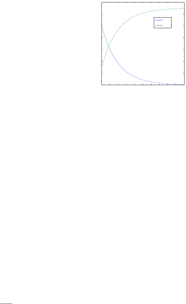
So we see that C
A
decays exponentially to zero, while C
B
rises exponentially
to its steady state; as an example see Fig 1.8. One of the great examples of
a first order reaction is radioactive decay, and this is why the abundance of
unstable isotopes (e.g.,
14
C,
235
U, ...) in a sample decays exponentially, and
this will be very important in the next section.
Problem 12: Just to be sure that you understand first order kinetics ... If the half
life of a substance that decays via first order kinetics is t
1/2
, how long do you have to wait
until 95% of the initial material has decayed? Explain why this question wouldn’t make
sense in the case of second order kinetics.
1.2. BOXES AND ARROWS TO DIFFERENTIAL EQUATIONS 45
Figure 1.8: Dynamics of the
concentrations in a first order
reaction A → B.
0 0.5 1 1.5 2 2.5 3 3.5 4 4.5 5
0
0.2
0.4
0.6
0.8
1
1.2
1.4
kt
concentration
C
A
(t)
C
B
(t)
What about the case A + B → C? If we take this literally as a mecha-
nism, we are describing a second order reaction, which means that A and B
molecules have to find each other in order to make C. The rate at which C
molecules are made should thus be proportional to the rate at which these
pairwise encounters are happening. What is this rate? If you imagine peo-
ple milling around at random in a large room, it’s clear that the number of
times per second that people run into each other dep ends both on how many
people there are and on the size of the room. If you follow one person, the
rate at which they run into people should go up if there are more people,
and down if the room gets bigger. Plausibly, what matters is the density
of people—the number of people divided by the size of the room—which is
just like measuring the concentration of molecules.
To obtain the rate of a second order reaction A+B → C, we thus need to
count the rate at which A molecules bump into B molecules as they wander
around randomly. By analogy with the people milling around the room,
if we follow one A molecule, the rate at which it bumps into B molecules
will be proportional to the concentration of B molecules. But then the total
rate of encounters between A and B will be proportional to the number of A
molecules multiplied by the concentration of B, so if we measure the number
of encounters per unit volume per second, we’ll get an answer proportional
to the product of the concentrations of A and B. Thus,
d[C]
dt
= k
2
[A][B]. (1.85)
Corresponding the to formation of C is the destruction of both A and B, so

46 CHAPTER 1. NEWTON’S LAWS, CHEMICAL KINETICS, ...
we must have
d[A]
dt
= −k
2
[A][B] (1.86)
d[B]
dt
= −k
2
[A][B]. (1.87)
The rate constant k
2
is now a second order rate constant, and you can see
that it has different units from the first order rate constant k in the equations
above; k
2
∼ 1/(time · concentration), conventionally 1/(M · s).
Perhaps the simplest second order reaction is A + A → B, for which the
relevant equations are
d[A]
dt
= −k
2
[A]
2
(1.88)
d[B]
dt
= k
2
[A]
2
. (1.89)
We have sen this equation before, describing the velocity of a particle that
experiences drag proportional to velocity squared. Thus we can proceed as
we did before:
d[A]
dt
= −k
2
[A]
2
d[A]
[A]
2
= −k
2
dt (1.90)
!
[A]
t
[A]
0
d[A]
[A]
2
= k
2
!
t
0
dt (1.91)
−
1
[A]
$
$
$
$
[A]
t
[A]
0
= −k
2
t (1.92)
−
1
[A]
t
+
1
[A]
0
= −k
2
t (1.93)
1
[A]
0
+ k
2
t =
1
[A]
t
(1.94)
[A]
t
=
[A]
0
1+k
2
[A]
0
t
, (1.95)
where [A]
t
is the concentration of A at time t, and in particular [A]
0
is the
concentration when t = 0. Thus the initial concentration does not decay as
an exponential, but rather as ∼ 1/t at long times; the time for decay to half
the initial value is t
1/2
=1/(k
2
[A]
0
) and depends on the initial concentration.
Notice that
[A]
t"t
1/2
≈
[A]
0
k
2
[A]
0
t
=
1
k
2
t
, (1.96)

1.2. BOXES AND ARROWS TO DIFFERENTIAL EQUATIONS 47
so that after a while the concentration is still changing, but the amount of
stuff we have left is independent of how much we started with (!).
Problem 13: Check that you understand each of the steps leading to Eq (1.95). As
a test of your understanding, consider the (rather unusual) case of a third order reaction,
in which three A molecules come together to react irreversibly. This is described by
d[A]
dt
= −k
3
[A]
3
. (1.97)
What are the units of the third order rate constant k
3
? Can you solve this equation?
time t
(minutes) [A]/[A]
0
[B]/[B]
0
0.25 0.7157 0.7635
0.50 0.7189 0.4305
0.75 0.5562 0.5262
1.00 0.4761 0.6195
1.25 0.4948 0.4876
1.50 0.3096 0.3169
1.75 0.3842 0.3702
2.00 0.2022 0.2764
2.25 0.1872 0.2613
2.50 0.1971 0.2738
Table 1.1: Two kinetics experiments.
Problem 14: Imagine that you do two experiments in chemical kinetics. In one
case we watch the decay of concentration is some reactant A, and in the other case the
reactant is B. The half lives of both species are about one minute, and perhaps because
you are in a hurry you run the reactions out only for 2.5 minutes. You take samples of the
concentration every quarter of a minute, and you get the results in Table 1.1. Perhaps the
first thing you notice is that the concentrations don’t decrease monotonically with time.
Presumably this is the result of errors in the measurement.
(a.) Can you decide whether the reactions leading to the decay of A and B are first
order or second order? Are A and B decaying i n the same way, or are they different?
(b.) Other than making more accurate measurements, how could you extend these
exp eri m ents to give you a better chance at deciding if the reactions are first or second
order?

48 CHAPTER 1. NEWTON’S LAWS, CHEMICAL KINETICS, ...
Figure 1.9: At the top, a re-
action scheme for the conver-
sion of B into D, using A as
a catalyst. At the bottom, this
scheme is written to make bet-
ter connections with the idea
of catalysis by an enzyme: E
is the enzyme, S is the ‘sub-
strate’ that gets converted into
the product P , and ES is a
complex of the enzyme and sub-
strate bound to one another.
The rate constants k
±
have the
same notation, but we write the
rate for ES → E+P as V , since
it’s the ‘velocity’ of the enzyme.
An important point about all this is that when we draw a more complex
reaction mechanism, each and every arrow corresponds to a term in the
differential equation, and the sign of the term depends on the direction of
the arrow. Consider, for example, the reactions shown at the top of Fig 1.9.
Really this is a scheme in which B is converted into D, and the A molecules
participate but are not consumed: the A molecules are catalysts. Notice
that there are three separate reactions, one for each arrow: A + B → C,
which occurs with a second order rate constant k
+
, C → A + B, which
occurs with first order rate k
−
, and C → D + A, with first order rate k. We
write k
+
and k
−
because these are forward and reverse processes.
Now we have to write out the differential equations, using the rule that
each reaction or arrow generates its corresponding term. Probably it’s eas-
iest to start with the equation for [C], since all three reactions contribute.
We see the arrow coming “in” to C from the left, which corresponds to the
concentration of C changing at a rate k
+
[A][B]. There is a second arrow
at the left, which corresponds to the concentration of C changing at a rate
−k
−
[C], where the negative sign is because the arrow points “out” and de -
scribes the destruction of C molecules. Finally, there is an arrow point out
to the right, which corresponds to the concentration of C changing at a rate
−k[C]. Putting all of these terms together, we have
d[C]
dt
=+k
+
[A][B] − k
−
[C] − k[C]. (1.98)

1.2. BOXES AND ARROWS TO DIFFERENTIAL EQUATIONS 49
For [B], only the k
+
and k
−
processes contribute:
d[B]
dt
= −k
+
[A][B]+k
−
[C]. (1.99)
Finally, for [A], all three reactions contribute, but with the opposite signs
from Eq (1.98):
d[A]
dt
= −k
+
[A][B]+k
−
[C]+k[C]. (1.100)
The important point here is not to solve these equations (yet), but rather
to be sure that you understand how to go from the pictures with arrows
describing the reactions down to the equations that describe quantitatively
the dynamics of the concentrations.
Notice that in Fig 1.9 we have also rewritten the scheme to make clear
that it describes an enzyme which converts ‘substrates’ S into ‘products’
P . In fact this is one of the standard schemes for describing biochemical
reactions, and it’s called Michaelis–Menten kinetics. To make contact with
the standard discussion, let’s call the concentration of substrates [S], the
concentration of products [P ], and so on. Then the kinetic equations become
d[S]
dt
= −k
+
[S][E]+k
−
[ES] (1.101)
d[ES]
dt
= k
+
[S][E] − (k
−
+ V )[ES] (1.102)
d[P ]
dt
= V [ES] (1.103)
d[E]
dt
= −k
+
[S][E]+(k
−
+ V )[ES]. (1.104)
You should notice that Eq’s (1.102) and (1.104) can be combined to tell us
that
d([ES]+[E])
dt
=0, (1.105)
or equivalently that [ES]+[E]=[E]
0
, the total enzyme concentration.
Solving all these equations is hard, but there is an approximation in which
everything simplifies.
Suppose that there is a lot of the substrate, but relatively little enzyme.
Then the high concentration of the substrate means that the binding of the
substrate to the enzyme will be fast. Although this isn’t completely obvious,
one consequence is that the concentration of the enzyme–substrate complex

50 CHAPTER 1. NEWTON’S LAWS, CHEMICAL KINETICS, ...
ES will come very quickly to a steady state; in particular this steady state
will b e reached before the substrate concentration has a chance to change
very much. But we can find this steady state just by setting d[ES]/dt =0
in Eq (1.102):
0=
d[ES]
dt
= k
+
[S][E] − (k
−
+ V )[ES] (1.106)
⇒ 0=k
+
[S][E] − (k
−
+ V )[ES] (1.107)
k
+
[S][E]=(k
−
+ V )[ES]. (1.108)
Now we use the constancy of the total enzyme concentration, [ES]+[E]=
[E]
0
, to write [E]=[E]
0
− [ES], and substitute to solve for [ES]:
k
+
[S][E]=(k
−
+ V )[ES]
k
+
[S]([E]
0
− [ES]) = (k
−
+ V )[ES] (1.109)
k
+
[S][E]
0
− k
+
[S][ES]=(k
−
+ V )[ES] (1.110)
k
+
[S][E]
0
=(k
−
+ V )[ES]+k
+
[S][ES] (1.111)
=(k
−
+ V + k
+
[S])[ES] (1.112)
k
+
[S][E]
0
k
−
+ V + k
+
[S]
=[ES]. (1.113)
The reason it is so useful to solve for [ES] is that, from Eq (1.103), the rate
at which product is formed is just V [ES], so we find
d[P ]
dt
= V [E]
0
k
+
[S]
k
−
+ V + k
+
[S]
, (1.114)
or
d[P ]
dt
= V [E]
0
[S]
[S]+K
m
, (1.115)
where K
m
=(k
−
+ V )/k
+
is sometimes called the Michaelis constant.
Equation (1.115) is the main result of Michaelis–Menten kinetics, and
it is widely used to describe real enzymes as they catalyze all sorts of re-
actions inside cells. What is this formula telling us? To begin, the rate
at which we make product is proportional to the concentration of enzymes.
Although we have written equations for the macroscopic concentration of
molecules, we can think of this in terms of what individual molecules are
doing: each enzyme molecule can turn substrate into product at some rate,
and the total rate is then this ‘single molecule’ rate multiplied by the total
number of enzyme molecules. In addition, Eq (1.115) tells us that is the

1.2. BOXES AND ARROWS TO DIFFERENTIAL EQUATIONS 51
substrate concentration is really low ([S] & K
m
), then the rate at which
catalysis happens is proportional to how much substrate we have; on the
other hand once the substrate concentration is large enough ([S] ' K
m
),
finding substrate molecules is not the problem and the rate of catalysis is
limited by the properties of the enzyme itself (V ).
Problem 15: The enzyme lysozyme helps to break down complex molecules built
out of sugars. As a first step, these molecules (which we will call S) must bi nd to the
enzyme. In the si m pl est model, this binding occurs in one step, a second order reaction
b etween the enzyme E and the substrate S to form the complex ES:
E + S
k
+
→ ES, (1.116)
where k
+
is the second order rate constant. The binding is reversible, so there is also a
first order process whereby the complex decays into its component parts:
ES
k
−
→ E + S, (1.117)
where k
−
is a first order rate constant. Let’s assume that everything else which happens
is slow, so we can analyze just this binding/unbinding reaction.
(a.) Write out the differential equations that describe the concentrations of [S], [E]
and [ES]. Remember that there are contributions from both reactions (1.116) and (1.117).
(b.) Show that if we start with an initial concentration of enzyme [E]
0
and zero
concentration of the complex ([ES]
0
= 0), then there is a conservation law: [E]+[ES]=
[E]
0
at all times.
(c.) Assume that the initial concentration of substrate [S]
0
is in vast excess, so that
we can always approximate [S] ≈ [S]
0
. Show that there is a steady state at which the
concentration of the complex is no longer changing, and that at this steady state
[ES]
ss
=[E]
0
·
[S]
[S]+K
, (1.118)
where K is a constant. How is K related to the rate constants k
+
and k
−
?
(d.) When the substrate is (N–acetylglucosamine)
2
, experiments near neutral pH
and at body temperature show that the rate constants are k
+
=4× 10
7
M
−1
s
−1
and
k
−
=1×10
5
s
−1
. What is the value of the constant K [in Eq (1.118)] for this substrate? At
a substrate concentration of [S] = 1 mM, what fraction of the initial enzyme concentration
will b e in the the complex [ES] once we reach steady state?
(e.) Show that the concentration of the complex [ES] approaches its steady state
exponentially: [ES](t) = [ES]
ss
[1 − exp(−t/τ)]. Remember that we start with [ES]
0
= 0.
How is the time constant τ related to the rate constants k
+
and k
−
and to the substrate
concentration [S]? For (N–acetylglucosamine)
2
, what is the longest time τ that we will
find for the approach to steady state?

52 CHAPTER 1. NEWTON’S LAWS, CHEMICAL KINETICS, ...
Figure 1.10: A cascade of enzy-
matic reactions.
Another interesting example is a sequence or cascade of reactions, as
schematized in Fig 1.10. Here we imagine that there is a molecule A which
can be stimulated by some signal to go into an activated states A
∗
. Once
in this activated state, it can act as a catalyst, converting B molecules into
their activated state B
∗
. The active B
∗
molecules act as a catalyst for C,
and so on. This sort of scheme is quite common in biological systems, and
serves as a molecular amplifier—even if we activate just one molecule of A,
we can end up with many molecules at the output of such a cascade.
One example that we should keep in mind is happening in the photore-
ceptor cells of your retina as you read this. In these cells, the A molecules
are rhodopsin, and the stimulation is what happens when these molecules
absorb light. Once rhodospin is in an active state, it can catalyze the acti-
vation of the B molecules, which are called transducin. Transducin is one
member of a large family of proteins (called G–proteins) that are involved
in many different kinds of signaling and amplification in all cells, not just
vision. The C molecules are enzyme called phosphodiesterase, which chew
up molecules of cyclic GMP (cGMP, which would be D if we continued our
schematic). Again, lots of cellular processes use cyclic nucleotides (cGMP
and cAMP) as internal signals or ‘second messengers’ in cells. In the pho-

1.2. BOXES AND ARROWS TO DIFFERENTIAL EQUATIONS 53
toreceptors, cGMP binds to proteins in the cell membrane that op en holes
in the membrane, and this allows the flow of electrical current; more about
this later in the course. These electrical signals get transmitted to other
cells in the retina, eventually reaching the cells that form the optic nerve
and carry information from the eye to your brain.
How can we describe the dynamics of a cascade such as Fig 1.10? Let’s
think about the way in which [B
∗
] changes with time. We have the idea
that A
∗
catalyzes the conversion of B into B
∗
, so the simplest possibility is
that this is a second order process: the rate at which B
∗
is produced will
be proportional both to the amount of A
∗
and to the number of available B
molecules, with a second order rate constant k
2
. Presumably there is also a
back reaction so that B
∗
converts back into B at some rate k
−
. Then the
dynamics are described by
d[B
∗
]
dt
= k[A
∗
][B] − k
−
[B
∗
]. (1.119)
There must be something similar for the way in which C
∗
is formed by
the interaction of B
∗
with C, and for simplicity let’s assume that all the
rate constants are the same (this doesn’t matter for the point we want to
make here!):
d[C
∗
]
dt
= k[B
∗
][C] − k
−
[C
∗
]. (1.120)
Actually solving these equations isn’t so simple. But let’s think about what
happens at very early times. In Eq (1.119), we can assume that at t = 0 we
start with none of the activated B
∗
. The external stimulus (e.g., a flash of
light to the retina) comes along and suddenly we have lots of A
∗
. There’s
plenty of B around to convert, and so there is an initial rate k[A
∗
]
0
[B]
0
,
which means that the number of activated B molecules will grow
[B
∗
] ≈ k[A
∗
]
0
[B]
0
t. (1.121)
Now we can substitute this result into Eq (1.120) to find the dynamics
of [C
∗
] at short times, again assuming that we start with plenty of [C] and
none of the activated version:
d[C
∗
]
dt
≈ k(k[A
∗
]
0
[B]
0
t)[C]={k
2
[A
∗
]
0
[B]
0
[C]
0
}t (1.122)
⇒ [C
∗
] ≈
%
1
2
k
2
[A
∗
]
0
[B]
0
[C]
0
&
t
2
(1.123)
So we see that the initial rise of [B
∗
] is as the first power of time, the rise of
[C
∗
] is as the second power, and hopefully you can see that if the cascade
54 CHAPTER 1. NEWTON’S LAWS, CHEMICAL KINETICS, ...
continued with C
∗
activating D, then [D
∗
] would rise as the third power of
time, and so on. In general, if we have a cascade with n steps, we expect
that the output of the cascade will rise as t
n
after we turn on the external
stimulus.
Many people had the cascade model in mind for different biological pro-
cesses long before we knew the identity of any of the molecular components.
The idea that we could count the number of stages in the cascade by looking
at how the output grows at short times is very elegant, and in Fig 1.11 we see
a relatively modern implementation of this idea for the rod photoreceptors
in the toad retina. It seems there really are three stages to the cascade!
This same basic idea of counting steps in a cascade has been used in very
different situations. As an example, in Fig 1.12, we show the probability that
someone is diagnosed with colon cancer as a function of their age. The idea
is the same, that there is some cascade of events (mutations, presumably),
and the power in the growth vs. time counts the number of stages. It’s
kind of interesting that if look only on a linear plot (on the left in Fig 1.12),
you might think that there was something specifically bad that happens to
people in their 50s that causes a dramatic increase in the rate at which they
get cancer. In contrast, the fact that incidence just grows as a power of age
suggest that there is nothing special about any particular age, just that as
we get older there is more time for things to have accumulated, and there
are several things that need to happen in order for cancer to take hold.
It’s quite amazing it is that these same mathematical ideas describe such
different biologic al processes occurring on completely different time scales
(years vs. seconds).
One can do a little more with the cascade model. If we think a little
more (or maybe use the equations), we see that the maximum number of
[B
∗
] molecules that will get made depends on their lifetime τ =1/k
−
: there
is a competition between A
∗
activating B → B
∗
, and the decay process
B
∗
→ B. This same story happens at every stage, so again the peak number
of molecules at the output will be proportional to some power of the lifetime
of the activated molecules, and this power again counts the number of stages
in the cascade, Thus the cell can adjust its sensitivity—the peak number of
output molecules that each activated input A
∗
can pro duce—by modulating
the lifetimes of the activated states. But if we change this lifetime , we also
change the overall time scale of the response. Roughly speaking, the time
required for the response to reach its peak is also proportional to τ. So we
expect that if a cell adjusts its gain by changing lifetimes, then the gain and
time to peak should be related to each other as gain ∝ t
n
peak
, where there
are n stages in the cascade; of course this value of n should agree with what

1.2. BOXES AND ARROWS TO DIFFERENTIAL EQUATIONS 55
Figure 1.11: Kinetics of the rod photoreceptor response to flashes of light. The data
p oints are obtained by measuring the current that flows across the cell membrane as a
function of time after a brief flash of light. Different shape points correspond to brighter
or dimmer flshes, and the response is normalize by taking the current (in pA, picoAmps;
pico = 10
−12
) and dividing by the light intensity (in photons per square micron). The
lowest intensity flashes give the highest sensitivity, but it’s hard to see the response at very
early time because it’s so small. As you go to brighter flashes you can see the behavior
at small times, but then as time go es on the response tends to saturate so what is shown
here is just the beginning. Solid line is r(t)=A exp(−t/τ)[1 − exp(−t/τ)]
3
, which starts
out for small t as r(t) ∝ t
3
. From DA Baylor, TD Lamb & K–W Yau, The membrane
current of single ro d outer segments. J Physiol 288, 589–611 (1979).

56 CHAPTER 1. NEWTON’S LAWS, CHEMICAL KINETICS, ...
Figure 1.12: Incidence of colon cancer as a function of age. The original data, collected
by C Muir et al (1987), refer to women in England and Wales, and are expressed as the
number of diagnoses in one year, normalized by the size of the population. At left the
data are plotted vs age on a linear scale, and on the right the are replotted on a log–log
scale, as in Fig 1.11. What we show here is reproduced from Molecular Biology of the
Cell, 4th Edition, B Alberts et al (1994). In the next version of these notes we’ll go back
and look at the original data.
we find by look at the initial rise in the output vs. time. A series of lovely
experiments in the 1970s showed that this actually works!
What’s nice about this example is that people were using it to think
about how your retina adapts to background light intensity long before we
had the slightest idea what was really going inside the cells. The fact that
simple models could fit the shape of the response, and that these models
suggested a simple view of adaptation, was enough to get everyone thinking
in the right direction, even if none of the details were quite right the first time
through. This is a wonderful reminder of how we should take seriously the
predictions of simple models, and how we can be guided to the right picture
even by theories that gloss over many details. Importantly, this works just
as well inside cells as it does for more traditional physics problems.
