
January 2018
Deferred Care
How Tax Refunds Enable
Healthcare Spending

About the Institute
The global economy has never been more complex, more interconnected, or faster moving. Yet economists,
businesses, nonprofit leaders, and policymakers have lacked access to real-time data and the analytic tools to
provide a comprehensive perspective. The results—made painfully clear by the Global Financial Crisis and its
aftermath—have been unrealized potential, inequitable growth, and preventable market failures.
The JPMorgan Chase Institute is harnessing the scale and scope of one of the world’s leading firms to explain the
global economy as it truly exists. Its mission is to help decision-makers—policymakers, businesses, and nonprofit
leaders—appreciate the scale, granularity, diversity, and interconnectedness of the global economic system and use
better facts, timely data, and thoughtful analysis to make smarter decisions to advance global prosperity. Drawing
on JPMorgan Chase’s unique proprietary data, expertise, and market access, the Institute develops analyses and
insights on the inner workings of the global economy, frames critical problems, and convenes stakeholders and
leading thinkers.
The JPMorgan Chase Institute is a global think tank dedicated to delivering data-rich analyses and expert insights
for the public good.
Acknowledgments
We thank our fantastic research team, specifically Kerry Zhang, Chenxi Yu, Peter Ganong, and Pascal Noel. This eort would not have
been possible without the critical support of the JPMorgan Chase Intelligent Solutions team of data experts, including Gaby Marano,
Stella Ng, Jacqueline Cush, and Bill Bowlsbey, and the JPMorgan Chase Institute team members Natalie Holmes, Sruthi Rao, Alyssa
Flaschner, Kelly Benoit, Caitlin Legacki, Courtney Hacker, Jolie Spiegelman, and Gena Stern.
We also would like to acknowledge with gratitude the invaluable input of academic experts who provided thoughtful comments,
including Jonathan Parker. For their generosity of time, insight, and support, we are deeply grateful.
Finally we would like to acknowledge Jamie Dimon, CEO of JPMorgan Chase & Co., for his vision and leadership in establishing the
Institute and enabling the ongoing research agenda. Along with support from across the Firm—notably from Peter Scher, Len Laufer,
Max Neukirchen, Joyce Chang, Steve Cutler, Patrik Ringstroem, and Judy Miller—the Institute has had the resources and support to
pioneer a new approach to contribute to global economic analysis and insight.
Contact
For more information about the JPMorgan Chase Institute or this report, please see our website www.jpmorganchaseinstitute.com
or e-mail institute@jpmchase.com.


2
Executive Summary
Healthcare represents a large and growing fraction of the US economy. Many policy strategies to control the rising cost of healthcare
have involved giving consumers more “skin in the game.” The reasoning behind many of these strategies is that if consumers’ choices
had a more direct impact on their own out-of-pocket spending, they would have more incentive to seek value for money, which in turn
would reduce costs for everyone. But what if consumers’ cash flow constraints prevent them from taking on higher out-of-pocket
costs in the short run, even when doing so would be better in the long run both for them and for the healthcare system overall?
The JPMorgan Chase Institute draws on its Healthcare Out-of-Pocket Spending Panel (HOSP) to investigate how a specific and
important cash infusion—a tax refund payment—drives the timing of out-of-pocket expenditures on healthcare. Consumers’ spending
on healthcare was significantly aected by cash flow dynamics. Even though they could likely anticipate the amount of the cash
infusion that their refund payment would bring, they did not increase their spending until the refund arrived; then, as soon as it
arrived, they immediately increased their spending.
Our analysis uncovers five key findings:
1. Consumers immediately increased their total out-
of-pocket healthcare spending by 60 percent in
the week after receiving a tax refund. Spending
remained elevated for about 75 days, during which
consumers spent 20 percent more out of pocket
on healthcare than before the tax refund.
2. In the week after the tax refund, out-of-pocket
healthcare spending on debit cards increased by 83
percent, and electronic payments increased by 56
percent. There was no change in credit card spending.
This suggests that liquidity from the tax refund
enabled the increase in healthcare spending.
3. In-person payments to healthcare service providers
represented 62 percent of tax refund-triggered additional
healthcare spending. This indicates that the timing
of a cash infusion aected when consumers received
healthcare, not just when they made a healthcare payment.
4. The tax refund caused consumers to make visits to
dentists’ and doctors’ oces and pay outstanding
hospital bills which they had deferred.
5. Cash flow dynamics had less eect on the out-of-
pocket healthcare spending patterns of consumers
who had higher balances in their checking account or
who had a credit card prior to the refund payment.
We conclude that cash flow dynamics are a significant driver of out-of-pocket healthcare spending. Even when consumers knew
with near-certainty the size and source of a major cash infusion, they still waited until the infusion arrived before spending. These
dynamics may shed light on ways insurers, healthcare providers, employers, and financial service providers could help consumers
receive care when they need it rather than when they have cash on hand to pay for it.

3
Introduction
Healthcare represents a large and growing fraction of the US
economy. Many policy strategies to control the rising cost of
healthcare have involved giving consumers more “skin in the
game.” The reasoning behind many of these strategies is that
if consumers’ choices had a more direct impact on their own
out-of-pocket healthcare expenditure, they would have more
incentive to seek value for money, which in turn would reduce
costs for everyone (Handel, 2013; Bhargava, Loewenstein,
Sydnor, 2017). But what if consumers’ cash flow constraints
prevent them from taking on higher out-of-pocket costs in the
short run, even when doing so would be better in the long run
for them and for the healthcare system overall?
In this study, we use a specific and important type of cash
infusion—a tax refund payment—to show that consumers’
spending on healthcare is significantly aected by cash flow
dynamics. Tax refunds are a significant cash flow event for
many households. In 2016, 73 percent of tax filers received a
tax refund, with an average refund of $2,860 (Internal Revenue
Service, 2017a).
1
When family members received this significant
cash infusion, they immediately increased their out-of-pocket
spending on healthcare. Furthermore, even though they likely
were able to anticipate the amount of the cash infusion as
soon as they had filed their returns, they did not increase their
spending until the refund actually arrived.
We draw on the JPMC Institute Healthcare Out-of-pocket
Spending Panel (JPMCI HOSP) data asset and examine how
healthcare payments vary in the days and weeks around
when account holders receive their tax refunds.
2
We analyze
average out-of-pocket healthcare expenditure on over a dozen
categories of healthcare goods and services for each day in the
100 days before and after a tax refund payment, for 1.2 million
checking account holders in the JMPCI HOSP who received a tax
refund between 2014 and 2016. This represents the first ever
daily event study documenting how families’ out-of-pocket
healthcare spending responds to the arrival of this significant
cash infusion.
3
Our analysis uncovers five key findings:
1. Consumers immediately increased their total out-of-pocket
healthcare spending by 60 percent in the week after receiving
a tax refund. Spending remained elevated for about 75 days,
during which consumers spent 20 percent more out of pocket
on healthcare than before the tax refund.
2. In the week after the tax refund, out-of-pocket healthcare
spending on debit cards increased by 83 percent, and
electronic payments increased by 56 percent. There was no
change to credit card spending. This suggests that liquidity
from the tax refund enabled the increase in healthcare
spending.
3. In-person payments to healthcare service providers
represented 62 percent of tax refund-triggered additional
healthcare spending. This indicates that the timing of a cash
infusion aected when consumers received healthcare, not
just when they made a healthcare payment.
4. The tax refund caused consumers to make visits to dentists’
and doctors’ oces and pay outstanding hospital bills which
they had deferred.
5. Cash flow dynamics had less eect on the out-of-pocket
healthcare spending patterns of consumers who had higher
balances in their checking account or who had a credit card.
Out-of-pocket healthcare spending
and ability to pay: Previous findings
and remaining questions
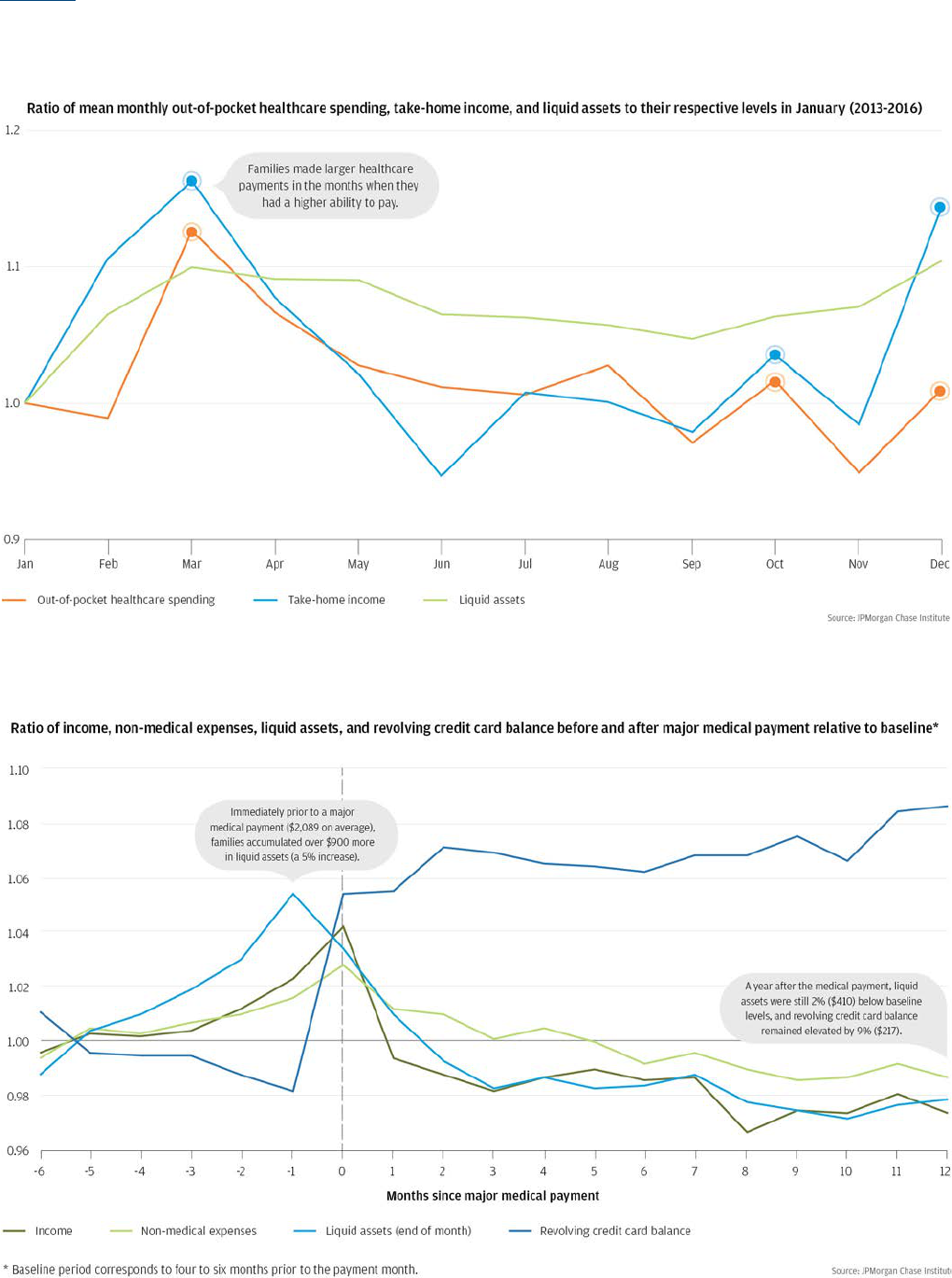
In previous research, the JPMorgan Chase Institute has shown
that account holders spend more out of pocket on healthcare
when they have more money. This is true even within a
single year. As shown in Figure 1, the average account holder
consistently spends more out of pocket on healthcare in
March and December; these two months are also consistently
marked by higher than average income (Farrell and Greig,
2017a). Furthermore as Figure 2 illustrates, account holders
timed major medical payments to occur in the same month as
increases in income and shortly after increases in liquid assets
(Farrell and Greig, 2017b).
4
DEFERRED CARE: HOW TAX REFUNDS ENABLE HEALTHCARE SPENDING
Introduction
Figure 1: Out-of-pocket healthcare payments and take-home income peak in March.
Figure 2: Account holders time major medical payments to coincide with higher income and bank balances.

5
DEFERRED CARE: HOW TAX REFUNDS ENABLE HEALTHCARE SPENDING
Introduction
The patterns in Figures 1 and 2 are striking because they suggest that cash flow dynamics may drive when families receive healthcare.
Still, important questions remain unanswered:
1. If family members are able to anticipate a cash infusion with near certainty, do they still wait for that infusion to arrive before
attending to their spending needs?
2. Do major healthcare payments follow increases in liquid assets because families time inflows to their needs, as opposed to
delaying spending until inflows arrive?
3. The months when income and out-of-pocket healthcare expenditure both tend to be highest (March and December) also happen
to fall during peak infectious disease season.
4
Could it be that people just need more healthcare at these times?
4. Even if cash flow dynamics aect when consumers pay for care, what does that mean for when they receive it? For example,
consumers might seek care when they need it, but then carry balances with healthcare providers until they have the cash to pay
down those balances. They might take advantage of volume discounts to stockpile medications and other supplies when income
is high, and then consume those stockpiles gradually as their needs dictate. In these cases, cash flow dynamics would drive when
consumers spend out of pocket on healthcare goods and services, but not when they get the benefits of those goods and services.
In this study, we address questions one through three directly, by observing out-of-pocket expenditures on healthcare in the days
around receipt of a significant cash infusion: a tax refund payment (Box 1). Account holders can anticipate the amount of their tax refund
payment almost perfectly once they file their returns, but they can neither control nor anticipate the precise timing of that payment.
Therefore, when we observe that increases in healthcare spending follow closely after receipt of the tax refund, we know that it is
implausible that families could have first planned the timing of the spending, and then timed the tax refund to immediately precede it.
We also know that it is implausible that family members coincidentally fall ill just as a tax refund payment arrives. As shown in Figure
3, the actual calendar date when a refund is received varies widely. Even the modal day in 2016 (February 10), accounted for only 3.8
percent of tax refund payments for that year. For dierent account holders, the 100 days before and after the tax refund payment
correspond to dierent points in the calendar, so there is no systematic relationship between days before or after the payment and
seasonal dynamics like infectious disease risk.
Figure 3. The timing of tax refund payments varies widely.
In order to address the fourth question, we separately analyze out-of-pocket healthcare payments to goods providers (for
example, drug stores or medical supply merchants) and to service providers (for example, doctors’ oces, dentists’ oces, or
hospitals). We further disaggregate payments to service providers that are made in person versus those that are made remotely,
based on administrative data that indicate whether a debit or credit card was physically present at the time of payment. Payments

6
DEFERRED CARE: HOW TAX REFUNDS ENABLE HEALTHCARE SPENDING
Introduction
made at the point of service are likely made at the time of service as well. Therefore, we infer in-person payments to healthcare
providers to represent services that were not received until the tax refund arrived. We characterize these payments as covering
costs of deferred care. In contrast, healthcare payments made remotely are likely to reflect payments made for services received
in the past and for which consumers were carrying unpaid balances. We describe the increase in remote payments after the tax
refund as deferred bill payments.
Box 1: Tax refunds are more than a convenient case study
Focusing on cash infusions that come specifically through tax refunds allows us to directly address important unanswered
questions. But tax refunds are not just a convenient case study. In previous research (Figure 1), we observed that out-of-
pocket healthcare expenditures were highest during tax refund season, which suggests that these payments may in fact
be a primary driver of expenditure on healthcare. Roughly three-fourths of tax filers receive a tax refund (IRS, 2017). The
average total tax refund in our sample was $3,100, which is 2.6 times the average payroll deposit.
5
This is a significant
amount of money to receive in a concentrated period of time. In 70 percent of cases, account holders received their entire
total tax refund on the same day. In 90 percent of cases, the entire amount arrived in multiple payments over the span of
a week or less. For 40 percent of account holders, a tax refund payment represents the largest single cash infusion into
their accounts for the whole year. Account balances are consistently highest on the day that the first tax refund payment is
deposited, as shown in Figure 4. For those whose capacity to spend out of pocket on healthcare is constrained by cash flow
dynamics, tax refund season is likely to be the time when those constraints are most alleviated.
Figure 4. Checking account balances in JPMCI HOSP increased by more than 50 percent when the first tax refund
payment was received.
Back to Contents

7
Findings
Finding
One
Consumers immediately increased their out-of-pocket healthcare spending
by 60 percent in the week after receiving a tax refund. Spending remained
elevated for about 75 days, during which consumers spent 20 percent more out
of pocket on healthcare than before the tax refund.
Figure 5 shows out-of-pocket healthcare spending in the JPMCI HOSP data asset in the 100
days before and after account holders received their first 2016 tax refund. The sharp
rise in the line on “day 0” indicates that spending increased immediately when the
refund payment arrived. Total healthcare spending was 60 percent higher in the
week after the refund payment, compared with a typical week prior to the refund.
This represents a significant departure from the stable pattern of spending over
the 100 days prior to the payment. The response to the cash infusion tailed o
after about 75 days, when spending returned to its pre-infusion pace. Over the
entire period of elevated spending, out-of-pocket healthcare spending was about
20 percent higher than a comparable period prior to the refund payment.
The arrival of the tax
refund triggered 75 days
of elevated out-of-pocket
spending on healthcare.
Figure 5. Consumers immediately increased their out-of-pocket healthcare
spending by 60 percent in the first week and 20 percent in the 75 days after
receiving a tax refund payment.

8
DEFERRED CARE: HOW TAX REFUNDS ENABLE HEALTHCARE SPENDING
Findings
The total additional spending represented in the shaded area of Figure 5 comes to about $30 per account in JPMCI HOSP. We infer
that this healthcare spending would have occurred at a dierent time if the tax refund payment had arrived at a dierent time
(see Box 2). Reflecting this inference, we will refer to these dollars as tax refund-triggered additional healthcare spending.
It is important to note that some of the tax refund-triggered additional spending is almost certainly for things that can wait. For example,
if a routine check-up occurs in March instead of January because a tax refund arrives in March instead of January, this may not be any
special cause for concern. In highlighting the fraction of spending for which the timing is determined by the arrival of cash, rather than
by customers’ needs or convenience, we are careful not to imply that every one of those dollars must necessarily be cause for concern.
Box 2: Computing tax refund-triggered additional healthcare spending
One way to quantify the impact of cash flow dynamics on out-of-pocket healthcare spending is with the following thought
experiment: “How much more did account holders spend on healthcare after the first tax refund payment arrived, compared
with what they would have spent on healthcare if their per weekday pace had carried on as it was prior to the refund payment?”
We identify the additional spending based on changes in the average per weekday pace of healthcare spending (rather than
average per day), because healthcare spending is naturally elevated on weekdays relative to weekends. Therefore, spending
will appear higher on “day 0” than the days around it, simply because tax refund payments always arrive on a weekday. We
sweep out this eect by adjusting each of the days to account for the fraction of account holders for whom that day falls on a
weekend.
6
Actual spending per person per day and our adjusted series based on the per person per weekday rate are shown
together in Figure 6. We use the adjusted series (in blue) to compute “tax refund-triggered additional spending.”
Figure 6. We adjust for weekend and weekday dynamics in computing “tax refund-triggered additional spending.”
Our computation of “tax refund-triggered additional spending” is represented graphically in Figure 7, which is a recasting of
the adjusted series (blue) in Figure 6. During any period, we can add up the heights of all the positive deviations (lighter bars),
and subtract the heights of all the negative deviations (darker bars), to arrive at a total number of “additional dollars” spent.
Over the period from day -100 to day -1, the cumulative additional spending comes to exactly $0 (by construction). Beginning
at day 0, cumulative additional spending increases until about day 75, when it stabilizes around $30.
Subject to the assumption that the jump in spending would have occurred on whatever day the tax refund arrived, the
additional spending can be described as “triggered” by the tax refund. This assumption is plausible given the extent to which
day 0 diers from all of the 100 days before it. The sense in which this spending is “triggered” by the refund refers specifically
to its timing; it does not refer to the economic concept of a marginal propensity to consume.
9
DEFERRED CARE: HOW TAX REFUNDS ENABLE HEALTHCARE SPENDING
Findings
Figure 7. “Additional healthcare spending” in each of the 100 days before and after the first tax refund payment
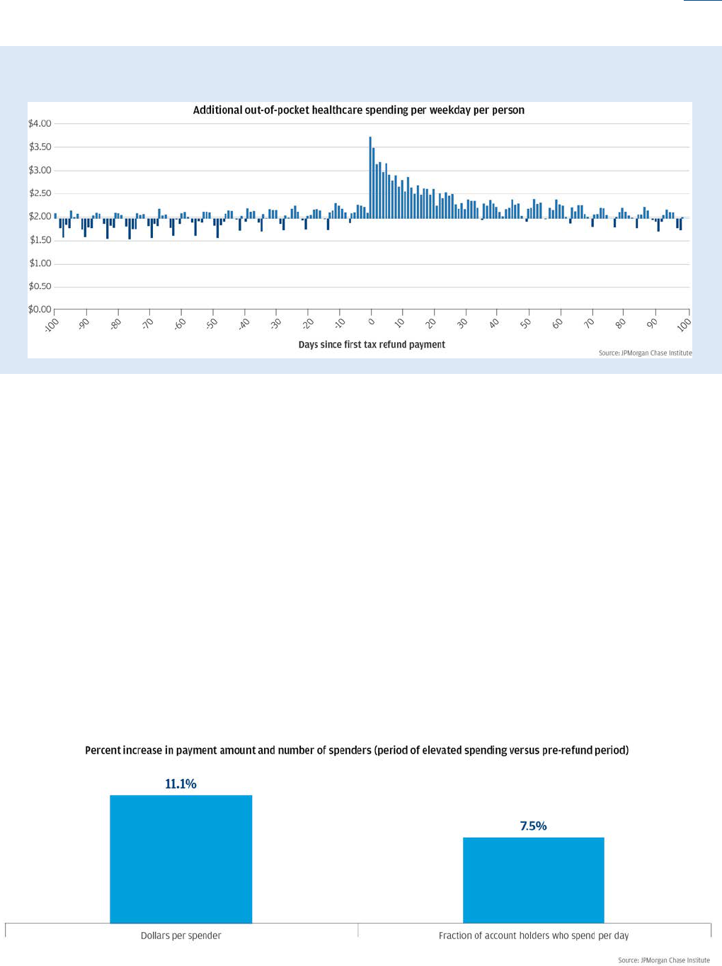
As shown in Figure 5, out-of-pocket healthcare spending remained elevated for roughly 75 days after the first tax refund payment was
received. Average spending per account was about 20 percent higher during this period than over a comparable period before the first
refund payment. This increase is driven by two dynamics—larger healthcare payments in a typical day, and more account holders making
healthcare payments in a typical day. The more powerful factor is the former, accounting for 59 percent of the tax refund triggered
additional healthcare spending.
7
As shown in Figure 8, the typical spender spent 11.1 percent more in a typical day during the period
of elevated spending, compared with the pre-refund period ($94 per day during the period of elevated spending, and $85 during the
pre-refund period). The other 41 percent of the increase is accounted for by the fact that the number of spenders on a typical day rises
from 2.3 percent of account holders during the pre-refund period to 2.5 percent during the period of elevated spending—translating to
a 7.5 percent rise (right bar in Figure 8).
We also observe that this increase in the average payment was driven in large part by an increase in the largest payment amounts
(account holders spending $150 or more in a single day). The cash infusion represented by a tax refund payment allowed more people
to make more purchases of healthcare goods and services, but, even more consequentially, it facilitated larger payments. This implies
that the cash infusion generated by a tax refund payment triggered additional spending on large healthcare ticket items that consumers
could have least aorded out of their pre-refund cash flow.
Figure 8. The number of consumers spending out-of-pocket on healthcare increased on a typical day after a tax refund was
received, and the average payment increased substantially.

10
DEFERRED CARE: HOW TAX REFUNDS ENABLE HEALTHCARE SPENDING
Findings
Finding
Two
In the week after the tax refund, out-of-pocket healthcare spending on debit cards
increased by 83 percent, and electronic payments increased by 56 percent. There
was no change to credit card spending. This suggests that liquidity from the tax
refund enabled the increase in healthcare spending.
Figure 9 disaggregates total out-of-pocket healthcare spending by payment instrument in the 100 days before and after account
holders receive their first tax refund payment. In the week following the arrival of the payment, out-of-pocket healthcare payments
on debit cards increased the most, by 83 percent. Spending via electronic payments also increased by 56 percent, but from a much
smaller base. By contrast, spending on credit cards did not change in response to the tax refund. Also striking is the degree to which
these patterns persist year after year (Figure 14 in the Appendix). In each of the three observed years, healthcare spending on
credit cards showed no change around the time of the tax refund, while debit card spending and electronic payments rose sharply.
The sharp rise in out-of-pocket healthcare spending on debit cards and electronic payments indicate that consumers had unmet
healthcare needs or unpaid healthcare bills, to which they waited to attend until after the cash arrived. Moreover the spending
response for healthcare is greater, in aggregate, than other types of spending: non-health spending on debit cards increased by 54
percent in the week after the tax refund (compared to 83 percent for health spending on debit cards).
The fact that the arrival of the tax refund triggers additional healthcare spending is striking because as soon as families file their tax
returns, they can anticipate with near certainty how much of a cash infusion to expect. If they had access to formal or informal credit
or to a cash buer, they could begin spending as soon as they learned the exact amount to expect. For example, one might expect
credit card spending to rise in anticipation of the refund payment. However, out-of-pocket healthcare spending on credit cards did
not increase either before or after the tax refund. For account holders who did not already know the amount of refund to expect,
the tax filing provided new information but no new liquidity; we see no evidence that this impacted spending behavior. Since filers
knew their tax refund amount when they filed, the refund payment itself provided new liquidity but no new information. The fact
that spending jumped in response to the refund payment, therefore, suggests that consumers were waiting for cash before making
healthcare payments, not just information about how much to expect.
Figure 9. Spending on debit cards increased 83 percent in the week after receiving a tax refund, with no osetting change
to credit card spending.

11
DEFERRED CARE: HOW TAX REFUNDS ENABLE HEALTHCARE SPENDING
Findings
Finding
Three
In-person payments to healthcare service providers represented 62
percent of tax refund-triggered additional healthcare spending. This
indicates that the timing of a cash infusion aected when consumers
received healthcare, not just when they made a healthcare payment.
Figure 10 disaggregates total out-of-pocket healthcare spending by payments made in person at healthcare service providers,
payments made remotely to healthcare service providers, and payments in any form (in-person or remote) to goods providers, in
the 100 days before and 100 days after account holders received their first tax refund payment.
8
Payments in person at service providers were 54 percent higher during the seven days after account holders received their first tax
refund payment than a typical week prior to the refund. Remote payments to service providers were elevated by 79 percent, but o
of a smaller base and for a shorter period of time than in-person payments. Payments to providers of stockable healthcare goods
increased by only 22 percent.
Figure 10. In the week of receiving a tax refund, in-person payments for healthcare service increased by 54 percent, and
remote payment of healthcare bills increased 79 percent.

12
DEFERRED CARE: HOW TAX REFUNDS ENABLE HEALTHCARE SPENDING
Findings
It is likely that payments made at the point of service are also made at the time
that the service is provided. This inference is supported by the sharper rise and
faster decay in remote payments in Figure 10. This likely reflects the fact that
consumers have more control over when they can make remote payments,
whereas in-person payments may require appointments to be made and
kept. Based on this inference, we conclude that the additional dollars spent
in person in Figure 10 go toward deferred care—healthcare services that
consumers would have received earlier, if their refund payment had come
earlier. In contrast, payments made remotely are likely to reflect payments
made for services that consumers had received in the past and for which they
were carrying balances (deferred bill payments).
The additional
spending triggered
by the tax refund went
disproportionately towards
in-person healthcare services
that that were likely deferred
from the period before
the refund arrived.
Figure 11 compares the distribution of the tax refund-triggered additional
spending to the distribution of total spending prior to the tax refund. We observe
that 62 percent of tax refund-triggered additional dollars were paid in person at
service providers (deferred care), a larger share than in the 100 days prior to the tax
refund (57 percent). Thirty-seven percent of tax refund-triggered additional healthcare
spending was paid remotely to service providers (deferred bill payments), compared to 33
percent before the tax refund.
Only 1 percent of tax refund triggered additional healthcare spending was paid to providers of healthcare goods
that can be stockpiled, like drugs or medical supplies, compared to 10 percent before the tax refund.
Figure 11: Most of the tax-refund triggered additional healthcare spending paid for deferred care.
Most consumers did not appear to use their tax refund to stock up on drug supplies and other healthcare goods. Rather, the additional
spending went disproportionately toward in-person healthcare services which were likely deferred from the period before the refund
arrived. We next explore what kinds of healthcare services were most likely to have been deferred.

13
DEFERRED CARE: HOW TAX REFUNDS ENABLE HEALTHCARE SPENDING
Findings
Finding
Four
The tax refund caused consumers to make visits to dentist and doctor oces
and pay outstanding hospital bills which they had likely deferred.
Dentists received a disproportionate share of the refund-triggered additional spending. Figure 12 illustrates that 32 percent of the
refund-triggered in-person payments to service providers went to dentists. By contrast, during the period prior to the tax refund
payment only 27 percent of in-person payments to service providers went to dentists (figures not shown). The refund-triggered
additional healthcare spending was less likely to go to doctors or hospitals, which, respectively, received only 23 percent and 6
percent of the additional spending triggered by the refund payment (compared to 27 percent and 7 percent of spending during
the pre-refund period respectively). The remaining 39 percent went towards other healthcare providers, including nursing service
providers, ambulance service providers, medical laboratories, opticians, optometrists, and chiropractors.
Remote payments for healthcare services (bill payments) mostly represented hospital bills even during the period before the tax
refund arrived; however, hospitals still received a disproportionate share of refund-triggered remote payments to service providers
(31 percent, compared with 28 percent during the pre-refund period). Twenty-one percent of refund-triggered additional remote
payments for services went to doctors and 6 percent went to dentists (compared to 19 percent and 15 percent respectively prior to
the tax refund, figures not shown).
In short, the tax refund triggered consumers to make visits to dentist and doctor oces and pay outstanding hospital bills which
they had likely deferred.
Figure 12. Dentist and doctor visits accounted for more than half of the deferred care that would have been received
earlier, if the tax refund payment had come earlier.

14
DEFERRED CARE: HOW TAX REFUNDS ENABLE HEALTHCARE SPENDING
Findings
Finding
Five
Cash flow dynamics had less eect on the out-of-pocket healthcare spending
patterns of consumers who had higher balances in their checking accounts or
who had a credit card before the payment arrived.
If consumers have access to formal or informal credit or a cash buer, they may be able to use
these tools to time spending more to their healthcare needs or to their convenience, rather
than to the arrival of a cash infusion. In Figure 13, we segment account holders on the basis
of their average daily checking account balances over the 100 days prior to their first tax
refund payment, and also on the basis of whether we observe any evidence that they had
a credit card prior to the first tax refund payment.
For consumers
who had less access
to liquidity, the tax
refund triggered a larger
increase in healthcare
spending.
We observe a clear gradient. Among account holders whose average daily checking
account balance was less than $536 (the lowest quintile), healthcare spending was 220
percent higher in the week after receiving the first tax refund payment compared with a
typical week prior to the refund payment. By contrast, for account holders with average
daily balances over $3,577 (the highest balance quintile), healthcare spending increased
by only 11 percent with the cash infusion. In other words, account holders with the lowest
checking account balances increased their out-of-pocket healthcare spending after the tax refund
by 20 times more than those with the highest balances. Similarly, healthcare spending increased more
sharply among those who did not have a credit card than among those who did (104 percent compared with 48 percent, respectively).
9
For consumers who had more spending power prior to the refund, the tax refund triggered a smaller increase in healthcare spending.
Figure 13. The cash infusion from a tax refund payment triggered a significantly sharper increase in healthcare
spending among account holders who had lower checking account balances or who did not have a credit card prior to
receiving their tax refund.
Back to Contents

15
Implications
Cash flow dynamics are a significant driver of out-of-pocket healthcare spending. Even when consumers likely know the size and
source of a major cash infusion, they still wait for the infusion to arrive before spending and begin spending immediately when it
does. Consumers in the JPMCI HOSP increased their out-of-pocket healthcare spending by 60 percent in the week after receiving a
tax refund. This spending would most likely have occurred earlier, if the refund payment had arrived earlier. This evidence on the
power of cash flow dynamics to drive behavior indicates opportunities for insurers, employers, healthcare providers, and financial
service providers to help consumers receive care when they need it, rather than when they have cash on hand to pay for it.
Cash flow dynamics drive when consumers receive healthcare, and not only when they pay for it. More than 60 percent of
tax refund-triggered additional healthcare spending was paid for in person and therefore likely represents care that consumers
would have received sooner, if the tax refund had come sooner. More than half of this care was provided by dentists and doctors.
Almost certainly, the timing of some of these services is not especially sensitive. However, we also observe that consumers who had
more spending power prior to the refund payment were less likely to time their spending based on when their tax refund arrived.
This implies that at least some consumers might otherwise prefer not to have the timing of their services determined by cash flow
considerations. The consequences to physical and financial health of deferring these services should be a target of empirical policy
research.
Health insurers and employers can play a role in helping people smooth their healthcare spending. Giving consumers “skin
in the game” may not be an eective way to control the rise of healthcare costs if consumers delay more cost-eective care (for
example, preventive or diagnostic services) due to short run cash flow constraints, only to require more costly interventions in the
long run. Therefore, strategies to curtail unnecessary healthcare utilization should not give consumers incentive to delay necessary
care because they are waiting for a cash infusion they know is coming. For example, insurers and employers could cooperate to oer
consumers who are enrolled in High Deductible Health Plans (HDHP) with an associated Health Savings Account (HSA) a mechanism
to allocate some of their tax refund directly to their HSA when they file their return, and even to begin spending from that allocation
before the refund payment arrives. Given that over a third of HSAs received no contributions in 2016 (Fronstin, 2017), employers
could more actively encourage and facilitate HSA allocations. For example, employees might be given an option to specify that HSA
allocations are automatically made from their paycheck on a regular basis, with built-in adjustments during periods of predictable
income spikes, like five-Friday months and bonus season.
Consumers’ willingness to enroll in a plan that includes an HSA may not just be driven by longer run considerations like deductibles
and premiums, but also by shorter run factors like whether covered services are paid for up-front or reimbursed later, and when
in the year contributions are made to HSAs. Understanding how consumers approach these tradeos can help inform the design of
innovative approaches to help people make the healthcare decisions that are best for their long run physical and financial health,
and for the sustainability of the system overall.
Patients and healthcare providers should take cash flow considerations explicitly into account when working together to
design an optimal healthcare plan. Our findings highlight the deep complexity that consumers and providers face in being active
partners in healthcare. For many consumers, this is not solely a question of working with their healthcare providers to align their
healthcare choices with their needs and financial resources. It is also a question of planning a care schedule so that out-of-pocket
costs line up with cash flow conditions. What care may be put o until an expected cash infusion arrives? For care that must not be
put o, how can the costs be covered in the meantime? Consumers need to understand both the health and financial consequences of
their choices in a dynamic framework where timing may sometimes be a critical component. Healthcare providers should prioritize
elements of a patient’s healthcare plan and oer clear medical advice around the consequences of delay.

16
Financial service providers have an opportunity to design
innovative products to meet the cash flow needs of consumers
and healthcare providers. Our findings indicate that tax refund
payments trigger consumers to immediately begin making
large healthcare payments which they had been deferring.
This suggests that financial service providers could design
innovative savings, credit, and payment tools (perhaps even
directly integrating these with planning and budgeting tools)
to give their customers more control over when and how to
cover large-ticket expenditures. These tools would likely be
useful even beyond healthcare. In the healthcare industry
specifically, a significant fraction of the tax refund-triggered
additional healthcare spending goes to paying down balances
with healthcare service providers. This indicates an opportunity to
cooperate with financial service providers to increase the amount
of care that can be extended and received when it is needed.
Cash flow dynamics are
a significant driver of out-
of-pocket healthcare spending.
This has important implications
for insurers, employers, healthcare
providers, and financial service
providers, to ensure consumers receive
healthcare when they need it, rather
than just when they have cash
on hand to pay for it.
Back to Contents


18
References
Barrow, Lisa and Leslie McGranahan. 2000. “The Eects of the Earned Income Credit on the Seasonality of Household Expenditures.”
National Tax Journal, Vol. 53, No. 4. Available at: https://ssrn.com/abstract=251094.
Baugh, Brian, Itzhak Ben-David, and Hoonsuk Park. 2014. “Disentangling Financial Constraints, Precautionary Savings, and
Myopia: Household Behavior Surrounding Federal Tax Returns.” NBER Working Paper no. w19783. Available at: https://ssrn.com/
abstract=2374558.
Bhargava, Saurabh, George Loewenstein, and Justin Sydnor. 2017. “Evaluating Health Insurance Decisions: Health Plan Choices from
a Menu With Dominated Options.” The Quarterly Journal of Economics. Volume 132, Issue 3 (August 2017): 1319–1372. https://dx.doi.
org/10.1093/qje/qjx011.
Broda, Christian, and Jonathan A. Parker. 2014. “The economic stimulus payments of 2008 and the aggregate demand for consumption.”
Journal of Monetary Economics. Volume 68, Supplement: S20-S36, https://dx.doi.org/10.1093/qje/qjx011.
Cilke, James. 2014. “The Case of the Missing Strangers: What we know and don’t know about non-filers” National Tax Association 107th Annual
Conference Proceedings, 2014. Available at: https://www.ntanet.org/conference/2014/11/107th-annual-conference-proceedings-2014/.
Farrell, Diana, and Fiona Greig. “Paying Out-of-Pocket: The Healthcare Spending of 2 Million US Families.” JPMorgan Chase Institute, 2017a.
Farrell, Diana, and Fiona Greig. “Coping with Costs: Big Data on Expense Volatility and Medical Payments.” JPMorgan Chase Institute, 2017b.
Handel, Benjamin R. 2013. “Adverse selection and inertia in health insurance markets: When nudging hurts.” The American Economic
Review 103, no. 7 (2013): 2643-2682. https://dx.doi.org/10.1257/aer.103.7.2643
Parker, Jonathan A. 2017. “Why Don't Households Smooth Consumption? Evidence from a $25 Million Experiment.” American Economic
Journal: Macroeconomics. Volume 9, number 4: 153-183. https://dx.doi.org/10.1257/mac.20150331
Fronstin, Paul. “Health Savings Account Balances, Contributions, Distributions, and Other Vital Statistics, 2016: Statistics from the EBRI
HSA Database” Employer Benefits Research Institute Issue Brief No. 438. September 2017. Available at: https://www.ebri.org/pdf/
briefspdf/EBRI_IB_438_HSAs.19Sept17.pdf
Internal Revenue Service (IRS). Filing Season Statistics for Week Ending Dec. 30, 2016. Internal Revenue Service, 2017a. Available at
https://www.irs.gov/newsroom/filing-season-statistics-for-the-week-ending-december-30-2016.
Internal Revenue Service (IRS). Filing Season Statistics for Week Ending Dec. 25, 2015. Internal Revenue Service, 2017b.
Molinari, Noelle-Angelique M., Ismael R. Ortega-Sanchez, Mark L. Messonnier, William W. Thompson, Pascale M. Wortley, Eric Weintraub,
Carolyn B. Bridges. 2007. “The annual impact of seasonal influenza in the US: Measuring disease burden and costs.” Vaccine. Volume 25:
(2007): 5086–5096. https://doi.org/10.1016/j.vaccine.2007.03.046
Blanton, Lenee, Noreen Alabi, Desiree Mustaquim, Calli Taylor, Krista Kniss, Natalie Kramer, Alicia Budd, Shikha Garg, Charisse N.
Cummings, Jessie Chung, Brendan Flannery, Alicia M. Fry, Wendy Sessions, Rebecca Garten, Xiyan Xu, Anwar Isa Abd Elal, Larisa
Gubareva, John Barnes, Vivien Dugan, David E. Wentworth, Erin Burns, Jacqueline Katz, Daniel Jernigan, Lynnette Brammer, “Update:
Influenza Activity in the United States During the 2016–17 Season and Composition of the 2017–18 Influenza Vaccine.” MMWR Morbidity
Mortality Weekly Report 2017. Volume 66: 668–676. http://dx.doi.org/10.15585/mmwr.mm6625a3
National Center for Health Statistics (NCHS). National Hospital Discharge Survey, 2010. Available at: https://www.cdc.gov/nchs/nhds/
about_nhds.htm
New York State Department of Health (NYSDH). Statewide Planning and Research Cooperative System (SPARCS), 2016. Available at:
https://www.health.ny.gov/statistics/sparcs/
Back to Contents

19
Endnotes
1 “Tax filers” are not the entire US population. In 2011, for
example, around 10 percent of the population may not have
been represented in any tax filing document, because their
households did not file a return with the IRS. Using other
administrative information, Cilke (2014) finds evidence that
most of the income of these non-filers comes from government
transfers. Nonetheless, for the small minority of the US
population who are non-filers, we do not know if they would
have received refund payments if they had filed, nor how
any such payments would have aected their out-of-pocket
healthcare spending behavior.
2 The JPMCI HOSP data asset was constructed using a sample
of de-identified core Chase customers for whom we observe
financial attributes, including out-of-pocket healthcare spending
between 2013 and 2016. For the purposes of our research, the
unit of analysis was the primary account holder. We focused
on accounts held by adults aged 18 to 64, as adults 65 and
older were more likely to make payments using paper checks,
which we could not categorize. To provide better visibility into
income and spending, we selected accounts which had at least
five checking account outflows each month, at least $5,000 in
take-home income each year, and used paper checks, cash, and
non-Chase credit cards for less than 50 percent of their total
spending. The JPMCI HOSP data asset includes customers who
resided within the 23 states in which JPMorgan Chase has a
retail branch presence. We re-weighted our population to reflect
the joint age and income distribution among the 18-64 year old
population within each state. See Farrell and Greig (2017a) for a
full description of the JPMCI HOSP data asset.
3 Other eorts to estimate the impact of tax refunds on consumer
spending have done so on a monthly basis and documented
higher total spending and specifically durable spending in
February among families eligible for the Earned Income Tax
Credit (Barrow and McGranahan, 2000). A number of studies
have measured the impacts of changes in tax rebates on
household spending with higher frequency. See Parker (2017)
and Broda and Parker (2014) for recent summaries of this
literature and evidence using Nielson Consumer Panel that
weekly household spending increased by 9-10 percent after
receiving the 2008 Economic Stimulus Payment. Notably, Baugh
et al. (2014), based on daily transaction data, provide evidence
that in the week following receipt of their tax refund, households
increase their restaurant spending by 8 percent, retail spending
by 12 percent and, ATM withdrawals by 16 percent.
4 The seasonality of influenza, which is a significant driver of
healthcare costs (Molinari, Ortega-Sanchez, et al., 2007), is
closely tracked by the US Centers for Disease Control and
Prevention. In the 2016/2017 season, influenza activity peaked
in late February, and prevalence fell sharply starting in the third
week of March (Blanton, Alabi, et al., 2017). Nationally, inpatient
discharges are consistently highest in March (NCHS, 2010) and
the daily rate of outpatient visits to hospitals in the state of New
York peak in March (NYSDH, 2016).
5 The average value of all tax refunds received in a year in the
JPMCI sample was $3,100; this includes directly deposited
federal and state tax refunds. This is roughly comparable
to national estimates. The average federal tax refund (i.e.,
not including state refunds) was $2,860 ($2,995 for directly
deposited tax refunds) in 2016, $2,797 ($2,957 for directly
deposited tax refunds) in 2015, and $2,792 ($2,918 for directly
deposited tax refunds) (IRS, 2017a; IRS, 2017b).
6 The cyclicality in the unadjusted (green) series in Figure 6 is
driven by the fact that healthcare spending on weekdays is
naturally elevated relative to weekends, and the fact that the IRS
does not distribute tax refund payments on weekends. As a
result, day 0 is a weekday for all 1.2 million accounts in our
sample, which therefore means that days 0+/- 7, 0+/- 14, and so
on also fall on weekdays for 100 percent of the sample. By
contrast, days 4+/-7, 4+/-14, and so on fall on weekends for 48
percent of the sample. Therefore, we compute the weekday-
adjusted (blue) series in Figure 6 as follows, for each day t:
Where x
t
is average out-of-pocket healthcare expenditure per
account on day t, x
p
is “typical” average daily expenditure per
account (where “typical” is identified by the 100 days prior to
the tax refund payment), and r
t
is the ratio of the fraction of
accounts for whom day t is a weekday to the “typical” fraction of
account-days that fall on weekdays (i.e., the 100 days prior to
the tax refund payment). Therefore, if day t is more likely to fall
on a weekday than is typical, then r
t
>1, so we adjust the average
for that day downward by a proportion of typical expenditure.
Conversely, if it is more likely to fall on a weekend than typical,
then r
t
<1, so we adjust the average for that day upward. Based
on this, we compute “tax refund-triggered additional spending”
over any period between day s and day t by:
Or, equivalently:
This reflects the fact that any dierence in average expenditure
in the period from day s to day t compared with an equivalent
number of days during the pre-refund period might be an
artifact of dierences in weekday versus weekend composition.
We use the r
τ
x
p
term in the summation above to sweep out that
artifactual component. Finally, we note that the adjusted (green)
series in Figure 6 is countercyclical with the unadjusted (blue)
series during the period prior to the refund payment. This
indicates that this approach somewhat over-corrects, in that it
20
“pushes” more expenditure from days that are most likely to fall
on weekdays to days that are most likely to fall on weekends.
This makes our approach conservative in the sense that it likely
underestimates the impact of the refund on the spike at day 0.
We also used an approach that computes seven separate
correction factors each of which inflates or deflates expenditure
on a day of the week, instead of a single weekday-versus-
weekend inflator. The results reported here were substantively
identical using this alternative approach. We also computed
additional spending using the actual (unadjusted) series, and
found all results to be substantively the same as what we have
reported here.
7 We decompose the growth in average spending per account
per day in logarithms. The natural logarithm of the ratio of
average daily spending during the 75 days after the refund
payment to average daily spending prior to the refund payment
(0.18) is itself equal to the sum of two logarithms. The first is
the logarithm of the ratio of the average payment sizes (0.11),
and the second is the logarithm of the ratio of the number
of payments (0.07). We use this to assign the “contribution”
of these two components to the overall growth in the
average—0.11/0.18, or 59 percent of the growth, is “contributed”
by growth in the average payment size, and 0.07/0.18, or 41
percent of the growth, is “contributed” by growth in the number
of payments.
8 Healthcare services include doctors, dentists, hospitals, nursing
service providers, ambulance service providers, medical
laboratories, opticians, optometrists, chiropractors, and “other”
healthcare services. Goods include all purchases at drug stores,
medical equipment suppliers, orthopedic goods and prosthetic
device suppliers, and hearing aid providers. Some overlap exists
between healthcare service providers and goods providers; for
example, a payment to an optometrist may be for a glaucoma
screening or for a pair of eyeglasses, or conversely a payment to
a drug store may be for a walk-in clinic visit.
9 We infer whether someone has a credit card on the basis of
whether we ever observe a credit card payment prior to the
arrival of the tax refund.
Back to Contents

Suggested Citation
Farrell, Diana, Fiona Greig, and Amar Hamoudi. "Deferred Care: How Tax Refunds Enable Healthcare Spending."
JPMorgan Chase Institute, 2018.

This material is a product of JPMorgan Chase Institute and is provided to you solely for general information purposes.
Unless otherwise specifically stated, any views or opinions expressed herein are solely those of the authors listed and may dier
from the views and opinions expressed by J.P. Morgan Securities LLC (JPMS) Research Department or other departments or divisions
of JPMorgan Chase & Co. or its aliates. This material is not a product of the Research Department of JPMS. Information has
been obtained from sources believed to be reliable, but JPMorgan Chase & Co. or its aliates and/or subsidiaries (collectively
J.P. Morgan) do not warrant its completeness or accuracy. Opinions and estimates constitute our judgment as of the date of this
material and are subject to change without notice. The data relied on for this report are based on past transactions and may not be
indicative of future results. The opinion herein should not be construed as an individual recommendation for any particular client
and is not intended as recommendations of particular securities, financial instruments, or strategies for a particular client. This
material does not constitute a solicitation or oer in any jurisdiction where such a solicitation is unlawful.
©2018 JPMorgan Chase & Co. All rights reserved. This publication or any portion hereof may not be reprinted, sold, or redistributed
without the written consent of J.P. Morgan. www.jpmorganchaseinstitute.com
