
AN ABSTRACT OF THE THESIS OF
Barbara R. Rowe for the degree of Doctor of Philosophy
in Family Resource Management presented on November 25,
1985.
Title:
The Economic Consequences of Divorce in Oregon
After Ten or More Years of Marriage.
Abstract approved:
,Redacted for Privacy
Alice Mills Morrow
The financial aspects of divorce are of great im-
portance to the growing numbers of men, women, and chil-
dren who live with the consequences of economic deci-
sions made at dissolution.
The purpose of this study
was to provide data on the economic aspects of
divorce
in Oregon after ten or more yearsof marriage; to de-
termine what assets were owned, how those assets were
valued for the purpose of division, which assets were
allocated to wives and which were allocated to husbands,
the factors that affected the allocation, and the effect
of asset division on the post-divorce economic well-
being of wives and husbands.
The sample was drawn from final divorce decrees
for marriages lasting ten or more years filed between
July 1983 and June 1984 in the Oregon counties of

Multnomah, Clackamas, and Washington.
Interviews were
conducted with 67 women and 49 men.
Most of these couples after ten or more years of
marriage, owned homes and tangible personal property,
most often furniture and a car.
Pensions were the most
frequently owned intangible personal property.
The
greater the value of an asset the more likely it was to
be valued objectively.
Assets were allocated fairly
equally between spouses.
However, this did not have the
effect of putting husbands and wives in similar economic
positions.
When predivorce and postdivorce household
incomes were compared, almost all of the movement toward
lower income was accounted for by wives.
Mothers were more likely than fathers to have cus-
tody of children.
When there were children under age
18, child support was usually awarded.
However, the
monthly amount of child support was less than one-half
of the estimated monthly cost of raising a child, lead-
ing to the conclusion that the custodial parent bears a
disproportionate share of the cost of raising a child.
While the allocation of property between divorcing
spouses is a concern that cannot be ignored, an equally
important concern in these marriages lasting ten or more
years is the lack of income-earning ability of the
wives.

Copyright by Barbara R. Rowe
December 30, 1985
All Rights Reserved

THE ECONOMIC CONSEQUENCES OF DIVORCE IN OREGON
AFTER TEN OR MORE YEARS OF MARRIAGE
by
Barbara R. Rowe
A THESIS
submitted to
Oregon State University
in partial fulfillment of
the requirements for the
degree of
Doctor of Philosophy
Completed November 25, 1985
Commencement June 1986

APPROVED:
Redacted for Privacy
Associate Professor of Family Resource Management in
charge of major
Redacted for Privacy
-/
Head of Department of Family Resource Management
Redacted for Privacy
titDean of Grate School
Date thesis is presented
-7-
November 25, 1985
Typed by Sandra Warren for
Barbara R. Rowe

ACKNOWLEDGEMENTS
I wish to especially thank Dr. Alice Mills Morrow,
my major professor, who gave up nights, weekends, holi-
days and vacations to see me through a Master's by-pass,
proposal, data collection, and dissertation.
Her cir-
tique of my research ideas and sharp editorial skills
have always made the finished product better.
I would also like to extend my sincere appreciation
to my graduate committee:
Dr. Arthur Gravatt, Dr. Gary
Tiedeman, Dr. Patricia Wells, and former committee mem-
ber Dr. Virginia Haldeman, for their support and con-
stant encouragement during my class work and the prepa-
ration of this dissertation.
A special debt of gratitude is owed Dr. Geraldine
Olson who served as the "guiding hand" throughout my
graduate program and research.
I was so lucky to have
her wise counsel and assistance.
Sincere appreciation is also extended to Ms. Evelyn
Leasher of Kerr Library, who kept an eye open for arti-
cles I could use in my research; Mr. Larry Gildea for
believing in me; Dr. Helen Berg of the Survey Research
Center, who helped me understand sampling techniques
and gave me a better grasp of research methods; Sandra
Warren for the thousand favors she did for me; and Mr.
Tom Gus, without whom my "n" would be half as big.
In addition, I wish to thank the men and women who

participated in this study for their time, and for the
deeper understanding they gave me of the divorce pro-
cess.
I can never repay my mother and my sister, Edith,
for their financial and moral support; nor my sister
Virginia, who provided ten months of free room, board,
and emotional support.
Lastly, a very special thank you to my children;
Alice, Tom, and Mike, without whose understanding and
love these years of graduate study would not have been
possible.

TABLE OF CONTENTS
Page
CHAPTER I
INTRODUCTION 1
Need for the Study
4
Statement of Purpose
5
Objectives of the Study 6
Delimitations of the Study 6
Limitations of the Study
6
Definition of Terms
7
Research Hypotheses 8
CHAPTER II
REVIEW OF LITERATURE 11
Divorce Law, In General
11
Property Division
15
Spousal Support
20
Child Custody and Child Support 26
Oregon Law
32
The Economics of Female-Headed Households
39
Loss of Economies of Scale
41
Poverty as a Result of Divorce
41
Public Assistance
43
Fewer Earners
45
Labor Force Participation
46
Summary
47
CHAPTER III
DESIGN OF STUDY AND METHODOLOGY
53
Development of the Instrument
53
Selection of the Sample
54
Collection of the Data
56
Data Analysis Procedure
57
Hypothesis One
58
Hypothesis Two
59
Hypothesis Three
59
Hypothesis Four
60
Hypothesis Five
61
Hypothesis Six
63
Summary of Statistical Analyses
65
CHAPTER IV
FINDINGS
66
Description of the Respondents
66
Representativeness of Respondents
66
Duration of the Marriage
68
Age of Divorcing Couples
69

Number of Minor Children
70
Sex of Petitioner
71
Characteristics of the Couples
73
Education
74
Employment
75
Assets
76
Income
77
The Settlement Process
79
Division of Property
82
Spousal Support
88
Decisions Pertaining to Children
90
Economic Well-Being After Divorce
94
Hypothesis Testing
98
Ownership of Assets
98
Dollar Value of Assets
102
Valuation of Assets
107
Allocation of Assets
110
Equitable Distribution
118
Post-Divorce Economic Well-Being
122
Summary of Statistical Analysis
132
Characteristics of the Sample
132
CHAPTER V
IMPLICATIONS AND RECOMMENDATIONS
138
Recommendations for Further Study
148
TABLE OF CASES
151
REFERENCES
152
APPENDIX A:
Introductory Letter
163a
APPENDIX B:
Court Data Collection Form
164a
APPENDIX C:
Research Instrument
165a

Table
4.1
Table 4.2
Table 4.3
Table 4.4
Table 4.5
Table 4.6
Table
4.7
Table 4.8
Table 4.9
Table 4.10
Table 4.11
Table 4.12
Table 4.13
Table 4.14
Table 4.15
LIST OF TABLES
Page
Analysis of variance of duration of
marriage for those who were inter-
viewed, those who were not inter-
viewed, and those who refused to
participate
68
Analysis of variance of wife's age
for those who were interviewed,
those who were not interviewed, and
those who refused to participate
69
Analysis of variance of husband's
age for those who were interviewed,
those who were not interviewed, and
those who refused to participate
70
Analysis of petitioner's sex for
those who were interviewed, those
who were not interviewed, and those
who refused to participate
72
Education levels of husbands
and wives
75
Employment of husbands and wives 76
Monthly income of husbands and wives
at the time of the divorce
78
Total household income prior to the
divorce 79
Comparison of responses for husbands and
wives regarding desire for the divorce.
80
Retention of family home
83
Estimate of division
87
Level of satisfaction with settlement 87
Attitude toward present economic
situation 95
Present household income of
respondents
96
Largest source of present income
97

Table 4.16
Attitude toward emotional situation ... 97
Table 4.17
Number of minor children for those who
owned other real property and those who
did not own other real property
99
Table 4.18
Ownership of intangible personal
property by wife's employment
history
101
Table 4.19
Ownership of intangible personal
property by wife's education level .... 102
Table 4.20
Correlations between selected
characteristics of divorcing couples
and the net dollar value of assets .... 106
Table 4.21
Methods of asset valuation used by
divorcing couples
109
Table 4.22
Wives keeping family home by custody
of children
112
Table 4.23
Husbands keeping family home by custody
of children
112
Table 4.24
Retention of other real property by
wife's age
113
Table 4.25
Retention of other real property by
marital duration
114
Table 4.26
Retention of other real property by
husband's employment
114
Table 4.27
Retention of tangible personal property
by children's custody
116
Table 4.28
Retention of tangible personal property
by who wanted divorce most at
the end
117
Table 4.29
Distribution of percentage of
assets to wife
120
Table 4.30
Percentage of assets to wife by owner-
ship of family home
122
Table 4.31
Multiple stepwise regression of selected
variables on post-divorce economic
well-being
125

Table 4.32
Respondent's attitude toward post-divorce
economic well-being by present
employment
126
Table 4.33
Respondent's attitude toward post-divorce
economic well-being by present
employment and sex
127
Table 4.34
Respondent's attitude toward post-divorce
economic well-being by whether couple made
decisions as to asset allocation
131
Table 4.35
Analysis of variance of respondent's
attitude toward post-divorce economic
well-being by whether couple made
decisions as to asset allocation and
sex
131
Table 4.36
Percentage of assets to wife by whether
couple made decisions as to asset
allocation and sex
132

THE ECONOMIC CONSEQUENCES OF DIVORCE IN OREGON
AFTER TEN OR MORE YEARS OF MARRIAGE
I. INTRODUCTION
Nationally, and in Oregon, there has been a dramatic
increase in the incidence of divorce (Gravatt and Hunt,
1979).
In a single year, 1981, 2,438,000 adults and
1,219,000 children, 2 percent of the total United States
population were affected by divorce (Statistical Abstract,
1982-83).
The 17,762 divorces and annulments in Oregon
in 1980 set a new record, and the rate per 1,000 was 6.8,
double what it had been in 1965 (Oregon Vital Statistics,
1980).
In human terms, a significant number of our popu-
lation has had a direct experience with divorce, either
in their own marriages or in their parents' or childrens'
marriages (Albrecht, 1980; Wiseman, 1975). The importance
of divorce lies not only in its numerical growth but also
in its increasing social, psychological, and economic
implications for families, individuals, and society
(McGraw, Sterin and Davis, 1982; Weitzman, 1981).
Since 1970, the number of families maintained by a
woman alone has increased by more than 53 percent to 9.4
million (Marital Status and Living Arrangements, 1983).
Female-headed families represent the largest subgroup of
the population living below the poverty level (Wattenberg
and Reinhardt, 1979). Most of the growth in female-headed
families has been related to increased marital disruption

2
and to the higher proportion of divorces which involve
children (Ross and Sawhill, 1975).
At least four studies have concluded that the poorer
a family is, the more likely the parents are to divorce
(Carter and Glick, 1970; Cutright, 1974; Glick and Norton,
1976; Goode, 1956). What is not known is the extent to
which divorced mothers are poor because they were poor
before the divorce and the extent to which they are poor
because of the divorce.
In all divorce actions, the court has a legal respon-
sibility to insure that the resolutions are equitable and
in the best interests of the parties (McGraw, Sterin and
Davis, 1982). Yet, very little is known about actual
awards and agreements. This lack of systematic informa-
tion makes it impossible for the parties, legislators or
the courts to make an accurate analysis of the impact of
divorce or to alter its effects.
There are five major decisions where divorcing cou-
ples may need to reach agreement: child custody, child
visitation, child support, alimony and division of prop-
erty (Kressel, Lopez-Morillas, Weinglass and Deutsch, 1978).
Recent studies using court records to analyze property
divisions have been "hampered by the fairly large amount
of missing information in the case record" (McGraw, Sterin
and Davis, 1982) or have been linked to state laws requiring
an equal division of community assets (Weitzman, 1981),
restricting the generalizations to a small minority of

3
jurisdictions.
For those cases in which information was
available, gender appeared to have an independent effect
on both the amounts and types of marital assets awarded
(i.e., wives usually received homes and furniture, hus-
bands received bank accounts, stocks, and businesses).
Most states, including Oregon, use the standard of
a "just" or "equitable" division of assets. This em-
powers the courts to distribute property regardless of
how title is held in order to achieve equity and justice
between the parties (Patterson, 1981).
This standard
allows a great deal of judicial discretion in the divi-
sion of marital property (Weitzman, 1981).
In addition,
Oregon law makes no distinction between assets acquired
before the marriage and those acquired after. Neither
is there any distinction regarding assets acquired after
the marriage by gift or inheritance.
The assets consid-
ered at dissolution are all of the property belonging to
either party or both parties, regardless of when or how
acquired, creating a "universal community" for division
(Cantwell, 1980).
Thus, Oregon is an ideal environment
for the collection of objective data regarding the prev-
alence and recipiency of property awards and for explor-
ation of the impact of property division on the post-
dissolution economic outcomes of divorcing families.

4
Need for the Study
The economic consequences of divorce are a major
social problem in the United States today.
Reforms which
were instituted in the 1970s have shifted the focus of the
legal process of divorce from moral questions of fault and
responsibility to economic issues of ability to pay and
financial need (Bahr, 1983; McGraw, Sterin and Davis, 1982;
Weitzman, 1981).
The increased importance of these finan-
cial issues suggests the need for more complete information
to aid judges, attorneys, and divorcing couples in making
economically sound decisions (Weitzman, 1981).
However, divorce as a primary subject of study has
been ignored to a great extent (Kitson and Raschke, 1981).
Prince-Bonham and Balswick (1980), in a decade review of
family literature, found that much of what we do know about
divorce has been a by-product of research on other topics
such as mental health and life satisfaction. Findings
based on these data sources provide more knowledge about
who divorces than what happens to them after divorce. Kit-
son and Raschke (1981), in a similar review, concluded that
one of the issues that needs to be addressed in future re-
search is analysis of the variables related to divorce ad-
justment, which include economic problems.
The numerous decisions and changes in life-style that
accompany most divorces present important challenges for
all the family-helping professions.
The economic aspects

5
of divorce are of great importance to the growing numbers
of men, women, and children who will live with the conse-
quences of economic decisions made at the time of dissolu-
tion.
Statement of Purpose
The purpose of this study is to provide data on the
economic aspects of divorce in Oregon after ten or more
years of marriage:
to determine how divorcing couples and
the courts value and allocate marital assets at dissolu-
tion; to look at the effects of marital duration, the ages
of the parties, their employment histories and earning
capacities, education levels, and the custodial and support
provisions of the decree on the valuation and allocation of
marital assets; and to determine whether or not the valua-
tion and division of marital property affects the post-
divorce economic well-being of husbands, wives, and their
children.
A study focusing on the financial aspects of divorce
settlements should provide information which will assist
divorcing couples, attorneys, the courts, and policy makers
concerned with the divorce process and the security and
economic well-being of families.
This information should also provide a frame of ref-
erence for developing educational programs and materials
in the areas of family economics and home management and
for strengthening marital, financial, and employment coun-

6
seling programs.
Objectives of the Study
The objectives of this study were:
1. to determine the types and total dollar
value of assets owned by divorcing couples;
2. to identify the methods used in valuing
assets for the purpose of division at
divorce;
3.
to identify types of assets allocated to
wives and types of assets allocated to
husbands;
4. to identify the factors affecting the types
of assets allocated to wives and the types
allocated to husbands;
5. to determine the percentage of the total
dollar value of assets allocated to wives
and the percentage allocated to husbands
at divorce; and
6.
to assess the effects of asset division on
the post-divorce economic well-being of
husbands and wives.
Delimitations of the Study
1.
The study is limited to the investigation of
divorces occurring after ten or more years of
marriage.
2.
The study is restricted to individuals granted
divorces in three Oregon counties.
Findings
can be generalized only to these respondents.
3.
The study is confined to those potential re-
spondents with a verifiable phone number and
address who agreed to be interviewed.
4.
The study is limited to divorces whose final
decrees were granted between July 1983 and
June 1984.
Limitations of the Study
1.
Potential respondents who declined to be inter-
viewed may be different from those who did
agree to be interviewed.
2.
Information provided by respondents is as
accurate as their recall will allow.

7
Definition of Terms
Assets - real and personal property:
real prop-
erty includes land and that which is affixed to it
(Black, 1983); personal property includes pensions,
stocks, bonds, and other investments, businesses, ve-
hicles, household durables, bank accounts, and life
insurance with a cash value.
Equitable distribution - for the purpose of this
study a division of assets is considered equitable when
either party receives no more than sixty percent or no
less than forty percent of the fair market value of all
assets legally and beneficially acquired during marriage
by either husband or wife, or both, regardless of legal
title.
Employment history
number of years in the labor
force, whether continuous or discontinuous, whether
part or full time paid employment.
Objective valuation - assets will be considered
objectively valued if some data were used to arrive at
a fair market value (e.g., independent appraisal, prop-
erty tax records, Blue Book, classified advertisements,
retirement account statements, bank statements).
Post-divorce economic well-being
defined for
this study by respondent's answer to the question, "Do
you think your economic situation now, as compared to
before the divorce, is better, somewhat better, about
the same, somewhat worse, or worse?"

8
Subjective valuation - assets will be considered
subjectively valued if no data were used to arrive at
a fair market value.
Types of assets - for the purpose of this study,
each asset has been placed into one of these four cate-
gories:
family home; other real property; tangible
personal property (e.g., cars, other vehicles,
fur-
niture and household durables) and intangible personal
property (e.g., bank accounts, stocks and bonds, pen-
sion and retirement benefits, life insurance, and
businesses or professional practices).
Research Hypotheses
Hypotheses for this study are as follows:
Hot:
The types of assets owned by divorcing couples
have no relationship to:
(a) age of wife
(b) age of husband
(c) duration of marriage
(d) employment history of wife
(e) employment history of husband
(f) wife's monthly income at time of divorce
(g) husband's monthly income at time of
divorce
(h) number of minor children
(i) ages of minor children
(j) education level of wife
(k) education level of husband
H 2:
There is no difference between the dollar value
0
of assets owned by divorcing couples and:
(a) age of wife
(b) age of husband
(c) duration of marriage
(d) wife's employment history
(e) husband's employment history
(f) wife's monthly income at time of divorce
(g) husband's monthly income at time of
divorce
9
(h) number of minor children
(i) ages of minor children
(j) education level of wife
(k) education level of husband
H
o
3:
There is no relationship between how assets are
valued for division and who retains the assets.
H
o
4:
There is no difference in the types of assets
allocated to wives and allocated to husbands by:
(a) age of wife
(b) age of husband
(c) duration of marriage
(d) employment history of wife
(e) employment history of husband
(f) wife's monthly income at time of divorce
(g) thusband's monthly income at time of
divorce
(h) number of minor children in wife's custody
(i) number of minor children in husband's
custody
(j) amount of child support paid per month
(k) amount of spousal support paid per month
(1) duration of spousal support
(m) who wanted divorce most in beginning
(n) who wanted divorce most at end
(o) education level of wife
(p) education level of husband
(q) whether or not the couple made the
decision(s)
(r) total dollar value of assets
H
o
5:
There is no relationship between equitable
distribution and:
(a) age of wife
(b) age of husband
(c) duration of marriage
(d) employment history of wife
(e) employment history of husband
(f) wife's monthly income at time of divorce
(g) husband's monthly income at time of
divorce
(h) number of minor children in wife's custody
(i) number of minor children in husband's
custody
(j) amount of child support paid per child
per month
(k) amount of spousal support paid per month
(1) duration of spousal support
(m) who wanted divorce most in beginning
(n) who wanted divorce most at end
(o) education level of wife
(p) education level of husband

10
(q) whether or not the couple made the
decision(s)
(r) whether or not a family home was owned
(s) whether or not other real estate was
owned
(t) whether or not tangible personal property
was owned
(u) whether or not intangible personal prop-
erty was owned
(v) total dollar value of assets
Hob:
The post-divorce economic well-being of husbands
and wives has no relationship to:
(a) age of respondent
(b) duration of marriage
(c) respondent's employment history
(d) thousehold income prior to divorce
(e) number of minor children with respondent
(f) amount of child support paid/received by
respondent
(g) amount of spousal support paid/received
by respondent
(h) if respondent wanted divorce most at
beginning
(i) if respondent wanted divorce most at end
(j) education level of respondent
(k) whether or not couple made the decision(s)
(1) net amount of assets received by respondent
(m) sex of respondent
(n) if respondent presently employed
(o) respondent's present household income

11
II.
REVIEW OF LITERATURE
Divorce Law, In General
Divorce law is closely related to a society's view
of marriage and the family (Clark, 1968).
The tradi-
tional view of marriage in the United States recognized
the husband as the primary decision maker who provided
economic support for the wife and children. The role
of the wife was caring for the household and children
(Glendon, 1980). Marriage was a permanent and cherished
union that the state had to protect and preserve.
The traditional view of divorce in the United
States was that a divorce could be obtained only if one
spouse committed a marital offense, such as adultery,
cruelty, or desertion, giving the other spouse a legal
basis, or grounds, for such action (Eisler, 1977).
Traditional divorce was based on an adversary proceeding
requiring that one party be guilty or responsible for
the divorce and the other be innocent (Kay, 1971).
Being found guilty or innocent had financial conse-
quences.
Only an innocent wife could receive alimony--a
means of continued support--and only a guilty husband
had to pay alimony (Crozier, 1935; Karowe, 1974).
Property awards were also linked to fault.
In most
states the court had to award more than half of the
property to the innocent party. This led to heated
accusations and counteraccusations of wrongs to obtain

12
a better marital settlement (Hogobloom, 1971).
At
divorce, the husband also remained responsible for the
children's economic support and all states gave prefer-
ence to a virtuous wife as the "natural and proper"
parent after divorce (Mnookin, 1975).
By the mid-nineteenth century, in the United States,
conservatives concluded that divorce was symptomatic of
a national moral crisis (Haien, 1980; Rheinstein, 1972).
Between 1884 and 1947, conservative reformers made many
efforts to abolish or stiffen traditional divorce laws
which were regarded as too liberal.
Since Congress could not be moved to propose an
amendment to the Constitution that would have extended
Federal legislative power to the field of family life,
conservatives began a parallel effort to restrict divorce
by coordinating state legislation.
To this end, the
National Conference of Commissioners on Uniform State
Laws was created.
At its first meeting, the body's
stated motive was to "stem the rising tide of divorce"
through "improvement and uniformity" of existing state
marriage and divorce laws (Rheinstein, 1972).
After the Commission's founding in 1892, the tra-
ditional view of marriage and divorce began to change.
It became generally agreed that dead marriages should
end, family assets should be fairly divided, economic
circumstances should govern alimony or maintenance, and
children, where possible, should know and associate with

13
both parents (Freed and Foster, 1983).
In 1965, the
Commission's co-chairmen suggested the abandonment of
traditional grounds for divorce and recommended that a
new approach to the administration of divorce laws be
researched and drafted (Rheinstein, 1972).
In 1967, the Ford Foundation granted funds to the
Commissioners to "assist in the research, deliberation,
and drafting necessary for promulgation of a comprehen-
sive family law" (Cheadle, 1981). Professor Robert J.
Levy of the University of Minnesota prepared a mono-
graphic study on marriage and divorce, which served as a
working basis for the Committee. In his report, Levy
concluded that American divorce law should be "predicated
solely and exclusively upon the ground of irremedial
marriage breakdown" (Rheinstein, 1972).
In 1970, the proposed Uniform Marriage and Divorce
Act (UMDA) was approved by the National Conference of
Commissioners (Rheinstein, 1972). In addition to adopt-
ing "no-fault" marriage breakdown as the sole ground for
divorce, it proposed new standards for alimony and prop-
erty division.
The Family Law Section of the American Bar Associa-
tion (ABA) withheld approval of the UMDA for four years.
The Bar attacked the statute on three grounds: the ease
and speed with which a divorce could be granted; the
absence of reconciliation provisions; and the proposed
provisions of the property distribution section (Podell,

14
1973). The ABA favored an "equitable distribution" pro-
vision giving divorce courts the power to distribute all
the property of the spouses, marital or separate.
Because of the ABA's objections, a section allow-
ing distribution of all property was written. This be-
came the provision "recommended generally for adoption"
by the ABA and is referred to in the UMDA as Alternative
A (Cheadle, 1981).
It provides that the property avail-
able for division is "the property and assets belonging
to either or both, however and whenever acquired, and
whether the title is in the name of husband, or wife,
or both" (Uniform Marriage and Divorce Act, 1982).
No
distinction is made between assets acquired before the
marriage and those acquired after marriage. Neither is
there any distinction regarding assets acquired by gift
or inheritance after the marriage. This permits the
broadest possible distribution of all assets held by
either spouse at the time of dissolution (Freed and
Foster, 1984). The essence of this alternative was
adopted by the Oregon Legislature in 1971.
The original guidelines providing for property
division were retained with minor changes as Alternative
B, because Commissioners from community property states
protested that their jurisdictions preferred to retain a
distinction between community and separate property
(Cheadle, 1981).
Alternative B describes marital prop-
erty as "all property acquired by either spouse after

15
the marriage except for property acquired
by gift, be-
quest, devise, or descent" (Uniform Marriage
and Divorce
Act, 1982).
This provision includes a presumption
that
all property acquired by either
spouse after the mar-
riage and prior to dissolution would
be marital property
"regardless of whether title is held individually
or by
the spouses in some form of co-ownership"
(Cantwell,
1980).
Both alternatives include other
factors to be
considered in making
a division, such as the contribu-
tions of the homemaker-spouse,
the custodial provisions
of the decree, and the economic circumstances
of each
spouse (Cantwell, 1980; Cheadle, 1981).
The Uniform Marriage and Divorce Act
met with exten-
sive criticism and was enacted by
only five states.
But
its basic concepts are
now incorporated in the statutes
of most states (Connell, 1981).
On July 1,
1985, South
Dakota became the fiftieth state to
adopt a form of no-
fault divorce (Americans for Legal
Reform, 1985; Freed
and Walker, 1985).
Regardless of the property distribu-
tion section, states have adopted
UMDA principles and
enacted legislation requiring the courts
to look beyond
title in deciding how much each
spouse should share in
the assets to be distributed (DiLeo and
Model, 1982).
Property Division
Historically, only two approaches
to dividing prop-
erty upon divorce existed:
the separate property system

16
of common law and the community of assets created in
community property jurisdictions.
Under common law, upon marriage, all the wife's
personal property became the property of her husband.
She did not lose title to real property owned by her
prior to the marriage, but her husband was entitled to
the rents and profits from her lands without account-
ability to her. If the marriage produced a child born
alive, the husband was entitled to income from his wife's
lands for the rest of his life.
During the marriage,
the wife could not sue or be sued on her own behalf; and
her husband was entitled to all of her earnings (Clark,
1968; Johnston, 1972).
In exchange, the wife received
the benefit of the husband's duty to support the family
in an amount determined by him. In addition, she was
entitled to one-third of the husband's real property if
she survived him (Bartke and Zurvalec, 1980; Karowe,
1974).
In the latter half of the nineteenth century, leg-
islation known as the Married Women's Property Acts was
passed in all of the common law states (Cheadle, 1981).
These laws gave women the right to own and control their
separate property, including their earnings from employ-
ment outside the home (Cantwell, 1980; Cheadle, 1981;
Kanowitz, 1969).
Traditional forms of joint ownership
continued, but if title was held in the name of one
spouse, that property was legally shielded from the other

17
(Cheadle, 1981).
These new freedoms did little to improve the eco-
nomic situation of most wives.
No property rights arose
during marriage by virtue of the marriage itself
(Krauskopf, 1976).
A spouse retained all the property
he or she earned or inherited during the course of the
marriage. The other spouse had no right or interest in
his or her partner's income or separate property (Weitz-
man, 1981). Upon divorce, real inequities existed if
the family assets had been acquired and held in the name
of the wage-earning husband (Wirth v. Wirth, 1971). The
courts had no power to order transfers or divisions of
separately held property (Krauskopf, 1976). Only joint-
ly held property was subject to distribution on dissolu-
tion (Greene, 1979).
In the community property jurisdictions, all prop-
erty owned by a married couple was classified as either
community property or separate property.
Separate prop-
erty consisted of all property owned by a spouse before
the marriage, any property obtained after the marriage
by way of gift or inheritance, and other property
acquired by a spouse during the marriage which could be
traced back to separate property (Cheadle, 1981; Greene,
1979). Each spouse retained the right to own, manage,
and control such separate property during the marriage
(Greene, 1979).
Community property consisted of all
other property acquired after marriage by either husband

18
or wife.
Each spouse owned a present, vested, undivided
one-half interest in the community property (Greene,
1979).
Despite the equality-of-sharing philosophy of com-
munity property laws, until recently, the husband had
the power to make virtually all management decisions in-
volving that property (Cheadle, 1981). He could sell
it, mortgage it, and in three states, give it away with-
out his wife's consent (Younger, 1973).
Any debt in-
curred by a married man was presumed to be a community
obligation and community property could be attached by
his creditors.
The wife needed to prove that she was
acting for the community in order to pay an obligation
from community assets (Karowe, 1974).
Upon divorce in community property states, the
court "disregarded" title and determined whether the
community owned the property or whether it was the sep-
arate property of one of the spouses (Patterson, 1981).
Each spouse was entitled to one-half of all the marital
property regardless of the monetary contribution each
person might have made towards its purchase (Krauskopf,
1975).
Separate property was generally not subject to
division, but remained with its original owner (Brake,
1982).
Today there are three general methods of dividing
property at divorce; the community property or "deferred"
community property approach, common law-title statutes,

19
and common law equitable distribution systems.
In community property states (Arizona, Arkansas,
California, Idaho, Louisiana, Nevada, New Mexico, Texas,
Washington, and the territory of Puerto Rico), property
is classified as either separate property or "marital"
property. Marital property is divided along the lines
of "equal in value" or "equitable."
The traditional
concept of fault has been abandoned, although in some
states (Arkansas, Idaho, Nevada, Texas, and Puerto Rico)
marital misconduct may decrease or eliminate the guilty
party's share of the community property (Freed and
Walker, 1985).
In the one common law-title state (Mississippi)
only jointly held property is distributed at divorce.
As to property not jointly held during the marriage,
the person with title during the marriage continues
ownership at divorce.
The remaining states (including Oregon) are equi-
table distribution states.
At divorce, courts permit a
spouse who has made contributions toward the acquisition
of property to claim an equitable interest in such prop-
erty, regardless of how it is titled (Freed and Walker,
1985). An increasing number of states recognize as con-
tributions being a homemaker and parent. Equitable dis-
tribution laws allow the courts to distribute property
according to the court's view of what is "equitable,"
taking into account the contributions of both parties,

20
regardless of the extent to which they were measured in
the marketplace (Foster and Freed, 1974).
Equitable
distribution does not guarantee any property interest to
a wife, but gives her the possibility of acquiring an
interest in the marital assets if the court views such
a decision as "just and proper."
Spousal Support
In traditional marriage, the primary obligation to
provide financial support to the family rested upon the
husband "so long as he is able" (Clark, 1968). This
duty was placed on the husband because at common law he
owned and controlled all his wife's property, all her
earnings, and her services. Even after the Married
Women's Property Acts permitted a wife control of her
separate property, it did not relieve the husband of his
duty to support her (Clark, 1968).
The same marital
rules functioned in the community property states,
except the wife's earnings, but not her separate prop-
erty, was subject to support obligations (Karowe, 1975).
This rule had limited practical significance in an
ongoing marriage for the courts refused in intervene
while husband and wife lived together (Kanowitz, 1969).
The wife had no legal recourse to require the husband
to provide support unless she left him and set up a
separate household (Krauskopf, 1977).
One explanation for the court's refusal to recog-

21
nize a remedy for the wife's right to support while the
parties lived together was that of keeping the parties
together.
In 1962, a New York court justified its re-
fusal to grant a support order to a wife who was still
living with her husband by saying, "The court should not
encourage a separation by granting temporary support in
which event the wife would move from the marital resi-
dence, if otherwise she might not" (Baker v. Baker,
1962).
Another purpose was the court's reluctance to
become involved "as budget makers for family units"
(Commonwealth v. George, 1948).
Private contracts be-
tween husband and wife which change the nature of his
support obligation have been ruled invalid on the theory
that "the duty of support is so important to the preser-
vation and stability of the marital relationship that
variation is against public policy and therefore void"
(Garlock v. Garlock, 1939).
There were some legal means through which third
parties would seek enforcement of support payments.
Under common law, while living with her husband, or
separated for good cause, the wife had the authority to
pledge his credit for the purchase of "necessaries" for
herself and the family (Clark, 1968).
This has been
described as the remedy afforded her if the husband
fails in his obligation of support (Ewell v. State,
1955).
This was actually a right available to the
creditor, not the wife.
She benefits only if she per-

22
suades the merchant to sell to her on the husband's
credit (Krauskopf and Thomas, 1974).
Poor laws or family responsibility statutes im-
posed an obligation upon certain persons to support
relatives.
In the tradition of Elizabethan poor laws,
these statutes were designed to secure minimum support
for the very poor.
They were not a remedy for enforce-
ment of the wife's common law right of support (Mandelker,
1956).
In essence, to attempt to obtain legal reinforce-
ment of the husband's duty to support, the wife had to
break up the family and seek a separation or divorce
decree.
If she chose to live with her husband, she
could, "in practice, get only what he chooses to give her"
(Citizens Advisory Council on the Status of Women, 1972).
In the United States, before and after The Married
Women's Property Acts were adopted, alimony could be
awarded upon absolute divorce even though the husband,
upon marriage, no longer acquired the property of his
wife.
Alimony awards have often been used to compen-
sate for the inequities of marital property law in
common law property states (Foster, 1978).
Such an
award "has always been inherently precarious.
It ceases
upon the death of the former husband and will cease or
falter upon his experiencing financial misfortune.
This
may result in serious misfortune to the wife and in some
cases will compel her to become a public charge"

23
(Rothman v. Rothman, 1974).
Under traditional divorce law, alimony was awarded
for the lifetime of either spouse or until remarriage
of the wife.
It was assumed that the wife had neither
the ability nor the resources to become self-supporting
(Foster, 1978). In 1979, the U.S. Supreme Court ruled
that wife-only statutes were based on sexual stereo-
types and were invalid, thus extending postdivorce
support to both partners (Orr v. Orr, 1979). As of
1984, forty-nine states have statutory provisions for
alimony, variously referred to as maintenance, allow-
ance, support, recovery, payment, separate maintenance,
and spousal support (Weitzman, 1981; Freed and Walker,
1985).
Alimony awards are still made through periodic
payments and are limited to the amount deemed "equitable
and just" (Karowe, 1974; Krause, 1981). The amount of
alimony awarded can be subject to modification or dis-
continuance upon a change in the earning capacity of
either spouse or other factors (Larson, 1979).
With the mounting dissolution rate, the advent of
no-fault dissolution, and the recent influx of women
into the labor force, the focal point of a spousal
support determination has shifted to the individual's
ability to become financially independent (Veith, 1978).
Advocates of divorce law reforms argue that the old laws
had converted "a host of physically and mentally compe-
tent young women into an army of alimony drones who...

24
become a drain on society and a menace to themselves"
(Doyle v. Doyle, 1957).
The aim of the new standards for alimony awards is
to provide support for spouses who (temporarily or
permanently) have compelling financial need (Weitzman
and Dixon, 1980; 1983).
This change has given rise to
the concept of rehabilitative alimony, also called
limited alimony or step-down spousal support.
Rehabil-
itative spousal support may be awarded for a period of
time during which the dependent spouse, usually the
wife, retrains for the job market.
This interim support
terminates automatically upon a date fixed in the final
decree of dissolution (Veith, 1978).
It should not be assumed that, historically, all
deserving wives received alimony (Foster, 1978).
In
fact, only a small percentage asked for or were awarded
alimony (Foster, 1978).
The U.S. Bureau of Census
reports that from 1822 to 1922, only 9 to 15 percent of
all divorces included provisions for alimony (Weitzman
and Dixon, 1980).
Today, alimony is awarded in less
than one-quarter of all divorces.
The national Commis-
sion on the Observance of International Women's Year
(1975) found that 14 percent of divorced wives surveyed
in a national poll said they were awarded alimony.
The
U.S. Bureau of the Census says that 15 percent of all
divorced or currently separated women in 1982 were
awarded alimony or maintenance payments or had an agree-

25
ment to receive them (Child Support and Alimony, 1983).
The amount of alimony typically awarded is too meager
to provide much economic protection for a dependent
spouse (Weitzman, 1981). In a random sample of 1977 Los
Angeles divorce decrees, Weitzman and Dixon (1980) found
the median alimony award was $209 per month.
The U.S.
Bureau of the Census reported that the mean total amount
of alimony received by women in 1981 was $3000 per year.
"After adjusting for inflation, this reflected a decrease
of about 25 percent from the 1978 level" (Child Support
and Alimony, 1983).
In order to determine whether awards had kept up
with the rate of inflation, Weitzman and Dixon (1980)
calculated the purchasing power of 1968 awards in 1977
dollars and vice versa, using the Consumer Price Index.
In Los Angeles, awards represented a real increase of
about $39 per month over the rate of inflation. Awards
in San Francisco, in contrast, had not kept up with the
rate of inflation.
Nonpayment of alimony and support obligations is
a widespread problem (Foster, 1978). Approximately 57
percent of alimony orders are violated (Child Support
and Alimony, 1983). Either no payment is made at all,
or payments are not made on time and arrearages build
up.
Even when payments are made for the first year or
two, they often stop or tail off with the passage of
time (Eckhardt, 1968; Foster, 1978). There is no other

26
area of law where court orders are so consistently vio-
lated (Foster, 1978).
Child Custody and Child Support
Initially in this country, child custody decisions
tended to follow English common law in that they con-
sidered the father to have the superior right to the
custody of his children, "and to the value of their
labor and services" (Derdeyn, 1976; Foster and Freed,
1978).
By the middle of the nineteenth century, there
was a gradual development of the belief that a child of
"tender years" required the care of the mother, and that
the child's best interests were served by awarding cus-
tody to the mother.
In the twentieth century, courts
are giving a substantial preference to the mother
(Mnookin, 1975).
This preference for maternal custody
was linked to the inclination of courts to award cus-
tody to the innocent party in a divorce action (Derdeyn,
1976; 1978).
Given the social convention that the wife
filed for divorce, the mother came to be the preferred
custodian (Foster and Freed, 1978; Mnookin, 1975).
The maternal preference standard was rarely ques-
tioned until the 1970's.
Social scientists began sug-
gesting that the legal standards of the time gave too
little weight to the psychological well-being of the
child and they called for "generally applicable guide-
lines" to govern all "child-placement disputes"

27
(Goldstein, Freud and Solnit, 1973).
This view has con-
tributed to recent legislative efforts toward sex-
neutral child custody statutes.
There is also a growing national trend toward
parents exercising joint custody of their children
(Folberg and Graham, 1979; Schulman and Pitt, 1982).
As of 1985, about 30 states had joint custody laws
which vary in substance and detail (Freed and Walker,
1985). Another recent phenomenon has been the enact-
ment of statutes in a growing number of states (in-
cluding Oregon) conferring upon a child's grandparents
legal standing to seek visitation rights with their
grandchildren after the divorce of the child's parents
(Freed and Foster, 1983).
A number of states have also
enacted laws criminalizing parental child abduction or
have put new teeth into their existing laws regarding
parental child abduction (Freed and Foster, 1984).
Today, in the majority of states, statutes impose
the obligation of child support on both parents (Freed
and Walker, 1985). Nevertheless, most courts continue
to place the major responsibility for postdivorce
support on the father (Derdeyn, 1978; Mnookin, 1981;
Weitzman, 1981). However, the amount of child support
payments is frequently small and many mothers receive
nothing at all (Espenshade, 1979). Yee (1979) reported
that child support orders entered by the Denver Dis-
trict Court during 1977-78 averaged $47.15 per month.

28
In a study conducted in 1972, Weitzman and Dixon (1979)
found that the median amount of child support ordered
for each child was $75 per month in Los Angeles. The
median total amount of child support per month per
family (for all children) was $121.
When these data
were compared to the estimated cost of raising two child-
ren to age 18 (Bureau of Labor Consumer Expenditure
Survey, 1960-61), the average child support awarded was
one-half of the direct cost of raising children in a
low-income family. Using data from a second sample,
drawn in 1977, they found that the median child support
award per child had risen to $100 per month and the
median total award had risen to $150. These amounts
had not kept up with the interim cost of living calcu-
lated at an increase of 8 percent per year. Nor were
they equal to half of the actual cost of raising a
child, even in a low-income family.
A 1972 report of
the Citizens Advisory Council on the Status of Women
concluded that "the data available indicate that pay-
ments generally are less than enough to furnish half of
the support of children," and that in most cases, ...
the mother is actually fulfilling a coextensive duty of
support to the child."
In California less than 10 percent of the child
support awards were tied to potential increases in the
father's income or to cost of living increases (Weitzman
and Dixon, 1979).
When the amount of child support re-

29
mains fixed, the payments are gradually consumed by in-
flation, and with each passing year, the mother assumes
an even greater share of the financial responsibility
for the children (Eden, 1979).
A large number of children never receive child
support awards in the first place. In a 1973 survey of
families receiving Aid to Dependent Children (ADC), ap-
proximately one-quarter of the mothers had child support
awards (Jones; Gordon, and Sawhill, 1976). In a 1975
survey of American women only 44 percent of the divorced
or separated mothers reported that they had been awarded
child support (National Commission on the Observance of
International Women's Year, 1975). In 1981, the Bureau
of the Census reported that of the 8.4 million families
with absent fathers, only five million were awarded
child support (Child Support and Alimony, 1983).
Many fathers are reluctant to live up to their
court-ordered support obligations (Collins, 1983;
Espenshade, 1979; Foster, 1978; Weitzman and Dixon,
1979). The first complete study of compliance with
child support orders was conducted by Professor Kenneth
Eckhardt in Wisconsin. Eckhardt (1968) found that in
the first year after the court order, 62 percent of the
fathers failed to comply fully with the order. Forty-
two percent did not make a single child support payment.
By the time ten years had passed, 79 percent of all
fathers had ceased providing any money. The Census

30
Bureau put the number of delinquents at over 2 million in
1981, 380,000 more than in 1978 (Child Support and Ali-
mony, 1983).
Recent years have brought new legislation aimed at
improving child support enforcement programs. The Uni-
form Reciprocal Enforcement of Support Act (URESA), ini-
tiated in 1950, permits the custodial parent to secure
support from the noncustodial parent residing in another
jurisdiction (Adams, 1983). Public law 93-647, passed
in 1975, established a federal parent locator service
to assist states in locating absent, non-supporting par-
ents (Uhr, 1979). And on August 16, 1984, Congress ex-
tended federal services to help enforce support in non-
welfare cases (Freed and Walker, 1985).
Typically, courts are lax in enforcing child sup-
port obligations (Collins, 1983; Espenshade, 1979).
There seems to be a general belief that a noncomplying
father simply does not have the means to support two
families.
In some cases a father's ability to support is
stretched to the limit by his remarriage and assumption
of the financial burdens of a new family. In other
cases, the husband's income is simply too low to share;
nothing divided by two is still nothing. Even husbands
who earn the average wage ... do not seem well off
enough to do without a large proportion of their income:
(Bane, 1976).

31
But Griffiths (1974), reporting to the U.S. House
of Representatives stated:
"We found no clear or consistent rela-
tionship between compliance with support
orders and absent parent's income.
Eighty-
two percent of the parents earning less
than $6,000 were not substantially complying
with their support orders or agreements- -
but neither were 66 percent of those earning
between $6,000 and $12,000, or 70 percent of
those earning $12,000 or more."
Winston and Forsher (1971), found that many
affluent fathers had evaded child support obligations
and that a number of physicians and lawyers had fam-
ilies who were ultimately forced onto welfare because
of the breakdown in enforcement of child support
orders.
They concluded that much middle-class poverty
is attributable to nonsupport by fathers who clearly
have the financial ability to comply with court orders.
And after a study of one small sample, Cassety
(1978) stated that an overwhelming majority of absent
fathers (86 percent) were "better off than their former
wives and children and even for many of the officially
poor mothers in the sample, enough money was available
to raise them above the poverty level without causing
the fathers to either fall below the poverty line or
to reduce their income level below that of their fam-
ilies."
She found only a small minority of the fathers
were truly unable to contribute anything toward the
support of their children while most could contribute
much more than the courts had believed possible.
She

32
concluded that "there appears to be an enormous untapped
source of funds that could be used to improve the eco-
nomic status of children in female-headed households."
Oregon Law
In 1971, Oregon became the second state to abolish
fault as the basis for dissolution of marriage and as a
basis for the award of spousal support and for the de-
termination of property settlements (Leo, 1972).
The
enactment of no-fault dissolution legislation was
hailed as a "realistic and generally rational approach
to an area of serious legal and social importance" (Leo,
1972).
Under earlier Oregon law, courts were required by
statute to make a disposition of real and personal prop-
erty as the courts deemed "just and proper in all cir-
cumstances" (Siebert v. Siebert, 1948).
Evidence of
fault, however, remained relevant to what constituted a
"just and proper" division of property (McCraw v. McCraw,
1962; Morgan v. Morgan, 1973).
"As this court has repeatedly and con-
sistently held in making a distribution of the
property of the marital community upon the
dissolution of a marriage, each case rests on
its own facts.
No formula can be stated, nor
percentage given, for all cases.
Each case
must be viewed independently, for a distribu-
tion which is just and proper in one case may
not be just and proper in another" (Johnson
v. Johnson, 1966).
This statute remained unchanged under Oregon's

33
Marriage Annulment and Dissolution Act of 1971, but evi-
dence of misconduct was no longer admissible.
Cases
decided under the 1971 act followed the property divi-
sion guidelines set out in Siebert v. Siebert (1948).
In Glatt v. Glatt (1979), the Oregon Court of
Appeals reaffirmed Siebert (1948) and stated, "the fac-
tors (that) ORS 107.105(1)(c) mentions with respect to
spousal support determination, while not controlling,
provide useful guidance in property divisions."
Those
factors were:
"(A) The duration of the marriage;
"(B) The ages of the parties;
"(C) Their health and conditions;
"(D) Their work experience and earning
capacities;
"(E) Their financial conditions, resources,
and property rights;
IT *
"(H) Such other matters as the court
shall deem relevant."
The court did not include (F) The provisions of the
decree relating to custody of the minor children of the
parties; or (G) The ages, health, and dependency condi-
tions of the children of the parties of either of them
(ORS 107.105 (1)(c)(A)-(H) (1974). Three years later,
the court said that "In practice, the financial portions
of a dissolution decree (spousal support, division of
property, and child support) are worked out together,
and none can be considered in isolation" (Grove v. Grove,
1977).
In 1977, the Oregon Legislative Assembly took

34
another step toward reform of the state's separate prop-
erty system in declaring that the contributions of home-
makers should be granted legal recognition in dividing
property and determining support awards (ORS 107.105(f)).
Under the 1971 Act, spousal support could be award-
ed to a party regardless of fault. The Act also delin-
iated factors for determining the amount and duration
of support: duration of the marriage, ages of the par-
ties, their health, their work experience and earning
capacities, their financial resources, the property and
custodial provisions of the decree, and the ages, health,
and dependency conditions of the minor children. The
trial court also retained discretion to considar addi-
tional factors which the court may deem relevant (ORS
107.105(1)(c); Stevenson, 1976).
In Grove v. Grove (1977), the Supreme Court dis-
cussed extensively the general questions surrounding
the award of spousal support. The court in Grove ac-
knowledged the interrelationship of spousal support,
property division, and child support (Stevenson, 1976).
On the question of duration of spousal support, the
court approved the general approach taken by the court
of appeals in Kitson v. Kitson (1974). To wit, when
there is a significant discrepency between a spouse's
probable future income and an income which would main-
tain the standard of living enjoyed during the marriage,
permanent spousal support is usually awarded (Grove v.

35
Grove, 1971). The court concluded that "the most sig-
nificant factor (in awarding support) is usually wheth-
er the wife's property and potential income, including
what she can earn or can become capable of earning will
provide her with a standard of living which is not
overly disproportionate to the one she enjoyed during
the marriage" (Grove v. Grove, 1977).
The court empha-
sized that it is not a comparison with the minimum
amount necessary to provide food, shelter, and other
basic necessities (Aarnas, 1978; Grove v. Grove, 1977).
ORS 107.105 was amended by the 1977 Legislative
Assembly to include two new factors for a court to con-
sider in awarding support.
"The need for maintenance,
retraining or education to enable the spouse to become
employable at suitable work or to enable the spouse to
pursue career objectives" and recognition of the home-
maker spouse "as an economic contributor to the marriage"
(ORS 107.105(1)(c)(H); ORS 107.105(1)(e), 1977).
The
1983 Legislative Assembly added several more factors to
be considered in awarding spousal support including the
contribution by one spouse to the education and earning
power of the other, the length of absence from the job
market by the dependent spouse and a realistic appraisal
of suitable job opportunities, the net spendable income
of the parties after assessing tax liabilities or bene-
fits, the costs of health care and life insurance premi-
ums, and the standard of living established during the

36
marriage (ORS 107.105(1)(d)(C)(F)(H)(J)(K)(L), 1983).
These changes also codified the Grove decision by in-
corporating the "not overly disproportionate to that
enjoyed during the marriage" standard (ORS 107.105 (1)
(d)(E)(M)).
In 1968, Tingen v. Tingen established factors to
be weighed in determining child custody, and held that
a party's misconduct is relevant only when it directly
affects the child's welfare (Tingen v. Tingen, 1968).
The 1971 Act eliminated the maternal preference statute
(Stevenson, 1976).
In Oregon, the court's primary con-
cern now is the "best interests of the child," with all
other matters being of secondary importance (In re Gaub,
1976; Ray v. Ray, 1972).
In 1981, Oregon's Supreme
Court rejected the use of tables or percentage methods
which were based on the noncustodial parent's income
alone as the appropriate means for determining the
amount of child support (O'Donnell, 1982).
By adopting
a "formula method," the court gave a clear directive
that both parents' incomes must be considered in deter-
mining the amount of support to be paid by the noncus-
todial parent (Smith v. Smith, 1981).
The formula re-
lating incomes of both parents to the child's needs
looks like this:
obligation of N =
income of N x needs of
income of N + income of C
children
where "N" represents the noncustodial parent and "C"

37
represents the custodial parent.
Criticism of the Smith
decision centered on the court's lack of guidelines in
determining the needs of the child leaving the trial
court to "decide whether ballet lessons, designer jeans
...or even the child's own room, are 'needs'"
(Allen,
1982; Smith, 1982).
Since 1977, bills have been introduced in every
biennial session of the Legislature proposing changes
in Oregon's divorce laws.
Many of these bills have been
spearheaded by the Women's Rights Coalition, which in-
cluded a dozen women's organizations, and the Oregon
Older Women's Caucus (Wohler, 1977).
In 1979, House
Bill 2648, a bill amending provisions relating to the
payment of child and spousal support and the division
of property, was defeated when the Coalition fell into
splinter factions in the face of heavy lobbying by a
divorced men's group (Williams, 1984).
Just before the
session ended, language mandating life insurance cover-
age on the obligor of child and spousal support was
written into another bill which did pass and became
Oregon law (ORS 107.820, 107.830).
The remaining sections of the bill were introduced
as House Bill 3177 in 1981.
Among its details were con-
siderations to be used in determining visitation rights,
the amount of child support, the support granted an ex-
spouse and additional grounds for
modifying a support
order should the obligor die prior to termination of the
38
support obligation (Turnquist, 1983). House Bill 3177
did not pass in 1981, but became the subject of an in-
terim study by the House and Senate Judiciary Committee,
clearing the way for final passage by the 1983 Legisla-
ture. As Senate Bill 12, the bill passed the Senate
almost unanimously and cleared the House with only ten
dissenting votes.
Governor Victor Atiyeh vetoed the
sections dealing with mandated joint custody, which had
been incorporated into the bill, and then signed Senate
Bill 12A-Engrossed into law on August 4, 1983 (ORS 107.
085, 107.105, 107.135, 107.407, 107.445, 107.820, and
ORCP 68C).
In 1985, the Legislative Assembly produced nearly
two dozen bills dealing with divorce issues: property
division, spousal support, child support, and child cus-
tody. The lobbying efforts of a fledgling political ac-
tion group called Dads Against Discrimination (DAD'S-
PAC) were aimed at creating a presumption favoring joint
custody (Hortsch, 1985).
It is not enough, in their
opinion, that state statutes or court decisions already
"encourage" joint custody, do award custody to some
fathers, and provide that neither parent shall have an
uncontested right to exclusive custody. Similar statutes
in other states have been vetoed on the grounds that
such statutes put the interests of the separating
spouses ahead of the best interests of the child (Freed
and Foster, 1983).

39
The Economics of Female-Headed Households
Between 1960 and 1982, there was a phenomenal
increase in the number of American families in which
only one parent, usually the mother, had the main
economic and social responsibility. The accelerated
growth in the number of one-parent families during
the 1970's--an increase of over 2.5 million--was far
greater than that of the preceding two decades.
The increasing prevalence of one-parent families
can be measured in terms of the proportion of children
living with only one parent (Ritagawa, 1981). Even
though the total number of children under 18 years old
in the United States declined by six million from 1970
to 1981, the number of children living with only one
parent rose by four million.
Thus, in 1980, one out of
every five children lived in a one-parent family
(Marital Status and Living Arrangements, 1983).
The
most prominent reason for the dramatic increase in the
number of one-parent families was the rising incidence
of divorce (Johnson, 1980; Ross and Sawhill 1975).
Accompanying the large increase in the number of
mothers maintaining their own families has been a
decline in the average age of female householders and
an increase in the number of families maintained by
women which contain young children. In 1979 there were
one million families with children under age six
maintained by women, and an additional 861,000 families

40
which had children under age six as well as children
ages six to 17 (Families Maintained by Female House-
holders, 1980).
One-parent families headed by women are more likely
than families maintained by men to be living at or
below the poverty level (Johnson, 1978; McEaddy, 1976;
Johnson, 1980).
Between 1965 and 1981, the number of
female - headed families living in poverty increased 70
percent while the number of all other poor families de-
clined 25 percent (Money Income and Poverty Status of
Families, 1982).
In 1981, the National Advisory Coun-
cil on Economic Opportunity said, "All other things
being equal, if the proportion of the poor who are in
female-headed families were to increase at the same
rate as it did from 1967 to 1978, they would comprise
100 percent of the poverty population by about the year
2000" (Caudle, 1982).
A number of explanations have been given why women
with children but without husbands find themselves in
such desperate economic straits: loss of economies of
scale; greater prevalence of divorce and death among
poor families; low and irregular levels of alimony,
child support and public assistance; fewer adult earn-
ers; fewer opportunities for female heads of families
to work; and lower wages than men when they do work
(Bane, 1976).

41
Loss of Economies of Scale
One economic fact of life is that it takes more
money to support two separate households than to sup-
port one household with the same number of people
(Vickery, 1978).
Economies of scale exist in rent,
furnishings, transportation, and food so that when
family members live together, the per capita cost of
maintaining a given level of living is less than when
living apart (Bane, 1976; Espenshade, 1979; Vickery,
1978).
When couples divorce these economic benefits
are reduced.
Emberson (1981), using revised data from
the U.S. Bureau of Labor, concluded that a four person
family consisting of husband, wife, and two children
would experience a 13 percent reduction in their level
of living if the parents divorced and set up separate
households.
Bane (1976) reported that "the loss of economies
of scale would in itself cause the proportion of child-
ren below the poverty level in female-headed families
to be approximately double that in male-headed families.
But in fact the proportion is six times greater, a much
larger difference than would be expected by economies
of scale alone."
Poverty as a Result of Divorce
Much of the decline in economic status experienced
by divorced mothers can be traced to the divorce (Bane,

42
1976; Brandwein, Brown and Fox, 1974). Kriesberg (1970),
in his study of mothers in poverty stated that "among
mothers who are husbandless due to separation or
divorce, whether or not they are poor is not related
to their socioeconomic status."
He indicated that in
addition to the poverty of many mothers prior to divorce,
a large number of previously non-poor wives and families
suffer downward economic mobility following divorce.
Using data from the Panel Study of Income Dynamics
(PSID), Hoffman (1977) compared the incomes of men and
women who stayed in intact families with the incomes of
men and women who were married in 1968 but divorced or
separated in 1974. Alimony and/or child support orders
were subtracted from the husband's income and added to
the wife's postdivorce income.
All income was calcu-
lated in constant 1968 dollars to examine changes in
real income. There was a sharp contrast in the economic
well-being of both men and women who were divorced by
1974. Divorced men lost 19 percent in real income while
divorced women lost 29 percent. Married men and women
experienced a 22 percent rise in real income during the
same period. To see what the income loss meant in terms
of family purchasing power, Hoffman and Holmes (1976)
constructed an index of family income in relation to
family needs. They found over the seven-year period
that the economic position of divorced men, when assess-
ed in terms of need, improved by 17 percent.
Over the
43
same period, divorced women experienced a seven percent
decline in terms of what their income could provide in
relation to their needs.
Weitzman (1981) used a similar procedure for cal-
culating the basic needs of the divorced couples she
interviewed in 1977. She assumed the basic needs level
for each family was the Lower Standard Budget devised
by the Bureau of Labor Statistics. Three lower stan-
dard budgets .were calculated for each family: one for
the predivorce family, one for the wife's postdivorce
family and one for the husband's postdivorce family.
She noted a substantive change in the two families' level
of living just one year after legal divorce.
Men ex-
perienced a 42 percent improvement in their postdivorce
level of living, while women experienced a 73 percent
loss. These figures may, if anything, underestimate the
disparity.
Weitzman assumed compliance with all alimony
and child support orders and included the full
amount of support ordered in the wife's income and sub-
tracted the full amount from the husband's income.
Where alimony or child support is not paid at all, or
is only partially paid, the husband's income will be
greater than assumed; the wife's less, and the income
difference between the two even greater.
Public Assistance
Another form of income available to divorced

44
mothers besides husbands' support payments is public
welfare.
How many divorced mothers turn to welfare is
difficult to determine. Wallerstein and Kelley (1980),
in their longitudinal study of 50 families following
divorce, noted that seven percent of the women moved
onto welfare rolls.
Goode (1956) reported that 26
percent of his sample felt that "public and community
agencies were the main source of financial aid during
economic difficulties."
In 1970, about "three-fifths
of the 3.4 million families with children headed by
women received welfare assistance (Stein, 1970). Hoffman
(1977) observed that, for women in the PSID sample not
receiving welfare in 1967, divorced females had a sub-
stantially higher chance of being on welfare in 1973
than did continuously married women. Mott and Moore
(1979) using data from the National Longitudinal Sur-
veys compared 449 women whose first marriages were
dissolved during the panel period (from 1968 through
1973) with a reference group who maintained stable first
marriages.
At the interview immediately following the
divorce, 23 percent were receiving some welfare com-
pared to three percent with stable marriages.
Since welfare payments are calculated to provide
only minimum subsistence income, benefits do not raise
families out of poverty (Brandwein, Brown and Fox, 1974).
Ninety-four percent of the 800,000 female-headed families
who had public assistance as their only source of income

45
in 1976 were living below the poverty level (Johnson,
1980). In almost half the states, welfare payments are
below the state's own determination of need (Wattenburg
and Reinhardt, 1979).
In some cases, the wife's own family appears to
be an important source of assistance.
In Goode's
(1956) study, 57 percent of divorcees reported their
families as the main source of financial aid during
crises.
Marsden (1969) observed that many mothers de-
pend upon relatives for regular income or special gifts
although Bernard (1971) found that barely one-third of
low-income mothers reported substantial assistance
from kin although most had some help from kin or friends.
These findings suggest that financial aid from the fam-
ily is more common and more substantial when middle-
income families divorce.
Fewer Earners
One obvious and important difference between one-
and two-parent families is in the number of income
earners.
Nearly all two-parent families with children
have at least one adult working full-time and about half
have two adult earners (Statistical Abstract, 1982-83).
In contrast, many single-parent families have no earn-
ers at all.
In 1980, more than 23 out of 100 families
headed by women had no earners, compared with 11 out of
100 husband-wife families (Johnson and Waldman, 1981).

46
For the divorced mother of very young children,
taking a job often conflicts with child care and home-
making.
Stein (1970) pointed out that the presence of
children and the lack of reliable child care often kept
female heads of families from full-time, year-round work.
As a result, the median income of women-headed families
with dependent children is one-third that of husband-
wife households.
Where the female family head has a
child under age six, her average family income is only
two-fifths of that for a household headed by a woman
with no youngsters (Levitan and Belous, 1981).
Labor Force Participation
Historically the employment and income situation
of females maintaining families has been bleak (Stein,
1970).
Most of the women are ill-equipped to earn an
adequate living for themselves or their families.
Single parents are often homemakers who are just enter-
ing or returning to the job market and must take on
employment in addition to child care (Smith, 1980).
Many cannot successfully compete in the labor market be-
cause of lack of sufficient education or training; ir-
regular and unstable work histories; age, sex or racial
discrimination in hiring; ill health; and the lack of
adequate and reliable child care (Stein, 1970).
Even so, divorced mothers, regardless of their
youngest child's age, were considerably more likely

47
than mothers in any other marital status category to be
in the labor force.
Despite their high labor force par-
ticipation rate, incomes of families maintained by women
remained low.
Part of the reason for the low average
incomes (and high unemployment rates) of women heading
families is their concentration in low-skill, low-paying
occupations.
In 1979, more than 72 percent of all em-
ployed women heading families were clustered in clerical,
service, and operative occupations (Working Women:
A
Databook; 1981).
Women employed in higher paying pro-
fessional, technical and managerial jobs tended to be
employed in traditional "women's occupations," such as
nursing and teaching school, while men in professional-
technical jobs were more likely to be in occupations
such as medicine, law, and engineering (Mellor and
Stamas, 1982; Milkovich, 1981).
Summary
In the past 15 years there have been significant
changes in family law; in state legislatures, in Con-
gress, and in the courts.
New divorce laws have re-
placed the old fault-based grounds for divorce.
Several
states simply added "irretrievable marital breakdown" or
"irreconcilable differences" to traditional divorce
grounds, some states have "marital breakdown" as the
sole ground, while other states allow divorce after a
period of "living separate and apart," either instead

48
of, or in addition to, no-fault grounds (Freed and Wal-
ker, 1985).
These laws assume that the acrimony and
bitterness surrounding divorce proceedings were created
in part by the adversarial process itself.
Therefore,
by eliminating fault, conditions would be created for
more rational and equitable financial settlements (Hogo-
bloom, 1970; Kay, 1971).
The majority of states now give the courts equi-
table power to distribute property upon divorce, either
in the form of real property or spousal support (Freed
and Walker, 1985).
This concept permits the contribu-
tions made by both spouses during the marriage to be
weighed against the net assets that are available at the
time of the divorce, regardless of title (Freed and Wal-
ker, 1985).
In a number of "equitable distribution"
states, "separate property" is not subject to distribu-
tion.
"Marital property," which is distributed, ex-
cludes either spouse's property by gift or inheritance
or property brought to the marriage (Dullea, 1985; Freed
and Walker, 1985).
The trend is to minimize marital
misconduct as a factor and base property awards on the
idea of marriage as a "economic partnership" with each
spouse having made an equal contribution.
The concept of alimony has also changed.
Di-
vorce reformers argued that it was outmoded to grant
lifelong support, especially since so many women were in
the labor force (Weitzman and Dixon, 1983).
To guide the

49
courts, many states' laws provide criteria for the court
to consider in its award of alimony, among them the
length of the marriage, the ages of the parties, their
contributions as a spouse, parent, wage earner, and
homemaker and their prospects for future employment.
But in general, the thrust of today's alimony standards
is to encourage formerly dependent spouses to assume
the responsibility for their own support (Weitzman and
Dixon, 1983).
The criteria for child custody reflects a new
equality between the sexes.
Current guidelines use
the "best interests of the child" standard.
The "tender
years" doctrine has lost ground and is rejected or rele-
gated to the role of "tiebreaker" in most states (Freed
and Walker, 1985).
Accordingly there has been an in-
crease in the number of awards of joint custody, and
also in the number of custody awards to fathers. In-
creasingly, provisions are being made that the wishes
of the child are to be considered in the court's deter-
mination (Freed and Walker, 1985). Child support laws
are also sex-neutral.
Both parents are equally respon-
sible for the financial welfare of their children after
divorce.
Today, a family headed by a woman is four-and-a-
half times more likely to be poor than the family of a
married couple or a family headed by a man (McCormack,
1985).
Even when they combine work with welfare and

50
other transfer payments, 36 percent of all families
maintained by women had incomes below the poverty level
in 1980, with children in more than four-fifths of
them (Hayghe, 1982; Levitan and Belous, 1981). Have
these recent changes in marital dissolution laws had
any effect on this situation?
Many wives enter into a dissolution with little
or no earning ability.
Even wives with full-time jobs
rarely earn as much as their husbands earn. A woman
who has not been employed or employed only on a part-
time basis may lack the marketable skills to improve
her financial position (Giele, 1983).
The continued
reliance on women as the principal caretakers of child-
ren after divorce often limits their working effort to
part-time and temporary employment (Perlman, 1976).
Current levels of spousal support do not offer
adequate economic protection to divorced women (Weitzman,
1981).
They are incompatible with the needs of women
whose earning capacities have been impaired in mar-
riages of long duration (Smith and Beninger, 1982).
Seal (1979) and Weitzman and Dixon (1980) found that
since no-fault laws went into effect in California,
alimony has been awarded less frequently and when award-
ed, the amounts, along with their duration, have de-
clined significantly.
There is no evidence that di-
vorce courts realistically evaluate the economic worth
of lost opportunity and nonmonetary contributions to a

51
marriage (Bahr, 1983; Smith and Beninger, 1982).
Before the passage of no-fault laws, wives typi-
cally received considerably more of the marital property
than husbands (Weitzman, 1981).
The current legal trend
is for property to be divided equally unless there is
some compelling reason not to do so (Bahr, 1983). When
equity is lacking in areas of employment opportunity
and childrearing responsibilities, even an equal divi-
sion of accumulated assets may be inadequate as a means
of achieving economic equality between husbands and
wives (McGraw, Sterin and Davis, 1982; Seal, 1980).
Clearly, recent changes in divorce laws have in-
creased the economic inequality between males and fe-
males.
Divorced females, but not divorced males, are
disproportionately represented among the poor and several
studies have documented that female but not male living
standards drop significantly after divorce (Espenshade,
1979; Weitzman, 1981).
In some states where equitable
distribution laws have gone into effect, bar associa-
tions and women's groups generally agree that the goals
of the laws are not being met and that revisions are
needed (Dullea, 1985). The problem with drafting re-
visions is that most divorce cases are settled by nego-
tiations in lawyers' offices and details of settlements
are difficult to obtain. Husbands, wives, attorneys
and the courts need to have more information concerning
the economic consequences of divorce in order to make

52
more enlightened decisions.

53
III.
DESIGN OF STUDY AND METHODOLOGY
This exploratory study sought to determine the
types and total dollar value of assets owned by divorc-
ing couples, to identify the methods used in valuing
assets at divorce, to identify the types of assets allo-
cated to wives and the types of assets allocated to hus-
bands, to identify the factors affecting the types of
assets allocated to wives and the types allocated to
husbands, to determine the percentage of the total
dollar value of assets allocated to wives and the percen-
tage of assets allocated to husbands at divorce and to
assess the effects of asset division on the post-divorce
economic well-being of husbands and wives.
This chap-
ter describes:
1) development of the instrument, 2)
selection of the sample, 3) collection of the data, and
4) data analysis procedure.
Development of the Instrument
A three part interview schedule was developed by
the researcher.
The first section aided the interviewer
in collecting data regarding the types and dollar values
of assets owned by divorcing couples and in determining
how assets were valued and divided at dissolution.
The
second section of the interview schedule included ques-
tions regarding the respondent's employment history and
the employment history of the former spouse.
The final

54
section of the interview focused on child custody and
support orders, current household incomes, education
levels, and their present employment status.
In addi-
tion to the interview schedule, data pertaining to the
parties' ages, duration of marriage, number and ages of
children, and sex of the petitioner were collected from
the divorce petitions filed in the offices of the Cir-
cuit Court Clerks in Multnomah, Clackamas, and Washing-
ton counties..
As the interview schedule was developed, the con-
tent was reviewed by faculty members of the Oregon State
University Family Resource Management Department.
It
was also submitted to the Oregon State University Sur-
vey Research Center for input on format, question word-
ing, and ease of analysis.
Prior to testing of the
interview schedule,
approval was sought and received
from the Committee for the Protection of Human Subjects
at Oregon State University.
A sample of fifteen divorc-
ed men and women from Benton county was used to pretest
the instrument.
Based upon the pretest and recommenda-
tions from the Family Resource Management Department,
the Survey Research Center and the researcher's graduate
committee members, changes were made to arrive at the
final form of the interview schedule (Appendix A).
Selection of the Sample
Individuals, married for ten or more years, whose

55
final decrees of divorce were granted in the Oregon
counties of Multnomah, Clackamas, and Washington between
July 1983 and June 1984, were designated as the target
population.
These three metropolitan counties make up
the majority of the Portland Standard Metropolitan Sta-
tistical Area (SMSA) which contains half of the state's
population.
In these three counties 2090 divorces were
granted in 1982 to couples married ten or more years
(Oregon Vital. Statistics, 1983).
The sample was drawn from final decrees of divorce
for marriages lasting ten years or more granted between
July 1983 and June 1984 in the Circuit Court Clerks
offices in each of the three counties.
Prior to col-
lecting data from the files, the county's record number
for each file was obtained from the Vital Statistics
Section of the Oregon State Health Division in Portland.
The counties' filing systems of the divorce decrees per-
mitted a systematic "1 in k" sampling procedure.
Based
on the number of divorces granted, a one in four inter-
val formula was used to provide a pool of 566 potential
respondents.
The number of potential respondents selec-
ted from each county was allocated proportionally to
population.
Fifty-three percent of the sample was se-
lected from Multnomah County, 23 percent from Clackamas
County, and 24 percent from Washington County. This
process made the sample self-weighted.
One hundred
forty-two men and women were contacted in Multnomah

56
County, 56 men and women were contacted in Clackamas
County and 79 men and women were contacted in Washing-
ton County.
It was believed that both male and female percep-
tions of asset division were needed to eliminate sample
bias in this study.
No effort was made to interview
both partners of each divorce because one of the parties
may be more willing to participate than the other.
Due
to the large number of the sample (254) having no veri-
fiable telephone number in the 1985 telephone directory,
all males and females having verifiable addresses and
telephone numbers were contacted by a letter telling
them about the study and asking for their participation.
A 66 percent non-response rate was expected based on the
experiences of researchers in Ohio (McCraw, Sterin and
Davis, 1982) and the pretest.
Collection of the Data
Potential respondents were sent personal letters
informing them of the study and asking for their par-
ticipation (Appendix B). Phone calls to make interview
appointments followed the letters, with a male caller
contacting men and a female caller contacting women.
The same-gender of the initial telephone contact was
deemed important to elicit positive responses unaffected
by inhibitions relating to gender (Warren and Rasmussen,
1977).

57
Appointments were made for interviews in the re-
spondents' homes or offices or in restaurants depending
upon respondent preferences.
Follow-up letters were
sent and calls made, as necessary, for difficult-to-
reach respondents.
After four unsuccessful attempts to
reach a potential respondent by telephone, at different
days and at different times of the day, the name was
dropped from the list of potential interviewees. New
addresses were sought for those letters returned to the
researcher as undeliverable by the postal service.
When
new addresses were located, letters requesting partici-
pation were remailed. Of the 566 potential respondents,
378 were not contacted because they had no verifiable
telephone number, letters were undeliverable, or they
could not be reached by telephone. Of the 188 contacted
by telephone, 116 were interviewed and 72 refused to be
interviewed resulting in a completion rate of 62 percent.
Information from the court records about marital
duration, ages of the parties, and numbers and ages of
children of the 378 men and women who were not inter-
viewed was compared with the 72 individuals who refused
to participate and the 116 who were interviewed.
Data Analysis Procedure
Data collected in the interviews was computer
coded to facilitate analysis.
A discussion of the pro-
cedures used to determine the rejection or nonrejection

58
of the null hypotheses follows.
All significance levels
were p<.05.
Each hypothesis is discussed separately.
The first step in data analysis was obtaining descrip-
tive statistics on the characteristics of the sample,
the settlement process, the decisions regarding prop-
erty valuation and division, the decisions pertaining
to child custody, child support and spousal support,
and the respondents' perceptions of well-being follow-
ing the divorce.
Hypothesis One
For hypothesis one, "t" tests and Chi square were
the statistical tools used. Hypothesis one stated that
there would be no relationship between the types of
assets owned by divorcing couples and the ages of the
parties, duration of marriage, employment histories of
the parties, their monthly incomes at the time of di-
vorce, the number and ages of their minor children, and
their education levels. The four types of assets con-
sidered were family home, other real property, tangible
personal property (e.g., cars, other vehicles, furniture
and household durables) and intangible personal property
(e.g., bank accounts, stocks and bonds, pension and re-
tirement benefits, life insurance, businesses or pro-
fessional practices, and any other asset). A "t" test
was used to compare the two groups, those who did own
the asset and those who did not, with the parties' ages,

59
years married, number and ages of minor children and
the parties' employment histories.
Chi squares com-
pared the two groups by the parties' incomes at the time
of the divorce and their education levels.
Hypothesis Two
ANOVA and Pearson's Correlation were used to test
the hypothesis that there would be no difference between
the net dollar value of assets owned by divorcing cou-
ples and the parties' ages, duration of marriage, em-
ployment histories of the parties, their monthly incomes
at the time of divorce, the number and ages of their
minor children, and their education levels.
A net
dollar value of assets was computed for each of the 116
couples by summing all of the asset values retained by
the wife and all of the asset values retained by the
husband.
The debts assumed by each party were then sub-
tracted from each value total. A correlation coeffi-
cient was calculated for each continuous independent
variable.
Analysis of variance was used to analyze the
parties' incomes and education levels as these variables
were measured categorically.
A Newman-Keuls test
followed each significant ANOVA to determine where the
differences existed.
Hypothesis Three
Hypothesis three stated that there would be no re-

60
lationship between how assets were valued for division
and whether husband or wife retained the asset.
For the
purpose of this study, two methods of valuation were
identified:
objective (if some data such as an indepen-
dent appraisal, property tax records, Blue Book, classi-
fied advertisements, retirement account statements or
bank statements were used) and subjective (if no data
were used to arrive at a fair market value). A 2x3 Chi
square was tabulated for each asset by its method of
valuation and whether husband had kept the asset, wheth-
er wife had kept the asset or whether the value of the
asset had been divided between them.
Hypothesis Four
Weitzman (1981) found "clear evidence of consistent
sex typing of various items of property" in her study.
Wives were more likely to be awarded the family home
and household furnishings, while husbands were more
likely to retain businesses and income-producing assets.
To determine if the same pattern existed in Oregon,
hypothesis four stated that there would be no difference
in the types of assets allocated to wives and allocated
to husbands. Each of the four types of assets (family
home, other real property, tangible personal property
and intangible personal property) were analyzed in re-
lation to who retained the equity in that asset; hus-
band or wife, or if the equity had been divided between

61
them.
ANOVA's were calculated to measure asset reten-
tion by the parties' ages, duration of marriage, the
number of children in each parent's custody, the amount
of child support, the amount and duration of spousal
support, their employment histories, and the net dollar
value of assets owned.
A Newman-Keuls followed each
significant ANOVA to determine where the differences
existed.
Chi squares were tabulated to measure asset
retention by the parties' monthly incomes at the time of
divorce, who wanted the divorce most at the beginning
and end of the divorce process, their education levels,
and whether or not the couple had made the decisions as
to asset allocation.
Hypothesis Five
Equitable distribution is a method of allocating
property upon divorce based on the concept that marriage
is a partnership or shared enterprise. Oregon law
states that all of the real or personal property of
either of the parties, or both, is to be divided as is
"just and proper in all circumstances" (ORS 107.105(e)
(f)). This standard veers away from an absolute 50/50
split, although that is often the goal unless there is
a showing of special circumstances. Hypothesis five
stated that there would be no relationship between equi-
table distribution and the ages of the parties, duration
of marriage, their employment histories, or their earn-

62
ing capacities.
These variables are the "factors...
which provide useful guidance in property divisions" to
Oregon courts and are found in statutory and case law
(Glatt v. Glatt, 1979; Grove v. Grove, 1977).
Other
variables included in this analysis were:
whether the
couple had made the decisions as to asset allocation,
who wanted the divorce most at the beginning and at the
end of the divorce process, the net dollar value of
assets owned,.and which types of assets were owned.
For the purpose of this study, a division of assets
was considered equitable when either husband or wife re-
ceived no more than sixty percent or no less than forty
percent of the fair market value of all assets.
To cal-
culate a percentage of assets, the total dollar value of
all assets owned by each couple was summed and their
debts subtracted to arrive at a net dollar figure.
Then
the value of all assets retained by each wife was summed
and the debts she assumed subtracted from her total.
These calculations were performed for each of the 116
families in the sample.
A percentage was then calculated
for each wife.
It was assumed that the husband received
the remaining percentage.
A correlation coefficient was
used to determine the strength of the relationship be-
tween the percentage of assets retained by wife and the
parties' ages, duration of marriage, their employment
histories, the number of children with each parent, the
amount of child support, the duration and amount of

63
spousal support and the net dollar value of assets.
Analysis of variance was used to measure percentage of
assets retained by the wife and the parties' incomes at
the time of the divorce, who most wanted the divorce at
the beginning and at the end of the divorce process,
their education levels, who made the decisions about
asset allocation and the four types of assets owned.
A
Newman-Keuls followed each significant ANOVA to determine
where the differences existed.
Hypothesis Six
For the purpose of this study, post-divorce econom-
ic well-being was determined by the respondent's answer
to Question 44 (Do you think your economic situation
now, as compared to before the divorce is: better,
somewhat better, about the same, somewhat worse or
worse?). It was believed that, in answering, the re-
spondent would take into consideration his/her age,
employment history, education level, household income
prior to the divorce, the number of children in his/her
care, the amount of child and/or spousal support the re-
spondent was paying or receiving, the number of years
married, if the respondent wanted the divorce most in
the beginning or at the end of the divorce process,
whether the couple had made the decisions as to asset
allocation, the net amount of assets received by re-
spondent, present employment status and present house-

64
hold income from all sources. Multiple regression was
used to estimate the relationship between the respon-
dent's answer and the independent variables.
A stepwise
method was used to determine which independent variables
would be included in the regression equation.

65
Summary of Statistical Analyses
Statistical
Data
Treatment
Characteristics Personal Data Descriptive
of Sample
Statistics
Hypothesis 1
Hypothesis 2
Hypothesis 3
Hypothesis 4
Hypothesis 5
Hypothesis 6
Types of Assets
Owned
Total Dollar
Value of Assets
ethod of
Valuation
Asset Allocation
"t" test
Chi square
Pearson's R
Analysis of Vari-
ance
Newman-Keuls
Chi square
Analysis of Vari-
ance
Chi square
Newman-Keuls
Percentage of
Pearson's R
Assets Allocated Analysis of Vari-
to Wife
ance
Newman-Keuls
Post-Divorce
Economic Well-
Deing
Stepwise Multiple
Regression

66
IV.
FINDINGS
This exploratory study sought to determine what
assets were owned by divorcing couples, how those assets
were valued for the purpose of division at dissolution,
which assets were allocated to wives and which were
allocated to husbands, the factors that affected the
percentage and type of assets allocated to wives and
allocated to husbands and the affect of asset division
on the economic well-being of wives and husbands after
divorce.
In this chapter, findings are discussed under
topics of:
1) description of the respondents, 2) the
settlement process, 3) division of property, 4) spousal
support, 5) decisions pertaining to children, 6) econom-
ic well-being after divorce, and 7) hypothesis testing.
Description of the Respondents
Representativeness of Respondents
The sample was drawn from final decrees of divorce
for marriages lasting ten or more years granted between
July 1983 and June 1984 in the Circuit Court Clerks'
offices in the Oregon counties of Multnomah, Clackamas,
and Washington. Based on a one-in-four systematic samp-
ling procedure, data were collected from court records
of 566 potential respondents.
The number of potential
respondents selected from each county was allocated pro-
portionally to population.
Fifty-three percent of the

67
sample was selected from Multnomah County, 23 percent
from Clackamas County, and 24 percent from Washington
County.
Two hundred fifty-four individuals from this
pool had no verifiable telephone numbers in the 1985
telephone directory and were not contacted. Three hun-
dred twelve individuals were sent letters explaining the
study and asking for their participation. One hundred
twenty-four individuals were unable to be interviewed
because their. letters were returned, their telephone
numbers had been changed since the directory printing,
or they were called four times and not reached. Seventy-
two individuals refused to participate in the study.
Interviews were conducted with 116 divorced individuals,
20 percent of the original sample. Of these, 67 inter-
views were with women and 49 interviews were with men.
Information from court records about duration of
the marriage, ages of the parties, numbers and ages of
children, and petitioner's sex was used as a basis of
comparison to determine if the 116 interviewed were
different from the 72 who refused to participate and
from the 378 individuals not interviewed.
Those who
were not interviewed were 254 individuals who did not
have a verifiable address plus 124 whose letters were
returned, their telephone numbers had been changed, or
who were unable to be contacted by phone after four
attempts.

68
Duration of the Marriage
There was a statistically significant difference
in the duration of the marriage between the three sample
groups.
Those who refused to be interviewed had mar-
riages of longer duration (18.9 years) than those who
were interviewed (17.2 years) and those who were not
interviewed (16.5 years) (F = 3,848, p = .0219) (Table
4.1). Also of note are the ranges of marital duration.
The sample was stratified to exclude any marriages in
which divorce had occurred before ten years so the min-
imum for each group was ten years. The maximum marital
duration for those who were interviewed and those who
refused to participate was 48 years. The maximum mari-
tal duration for those who were not interviewed was 49
years.
Table 4.1.
Analysis of variance for duration of mar-
riage for those who were interviewed, those
who were not interviewed, and those who
refused to participate.
Source
Sum of
Mean
Squares DF Squares Ratio Prob.
Between Croups
375.6222
2 187.8111 3.848 .0219
Within Groups 27234.3493 558 48.8071
Total 27609.9715 560
F*=3.848 with 2,558 d.f., do not reject at the .05 level
of significance

69
Age of Divorcing Couples
The average age of wives who were not interviewed
was significantly younger (38.2 years) than the average
age of wives of both the wives interviewed (40.3 years)
and the wives who refused to participate (41.1 years)
(F = 4.919, p = .0076) (Table 4.2).
The range of wives'
ages in the non-interviewed group was 25 to 70 years,
28 to 73 years in the interviewed group, and 27 to 85
years in the group who refused to participate.
Table 4.2. Analysis of variance of wives' ages for
those who were interviewed, those who were
not interviewed, and those who refused to
participate.
Source
Sum of Mean
Squares DF Squares Ratio Prob.
Between Groups 754.0523 2 377.0262 4.919 .0076
Within Groups 42537.8760
555 76.6448
Total 43291.9283 557
F*=4.919, with 2,555 d.f., do not reject at the .05
level of significance
Similarly, husbands in the group not interviewed
were significantly younger (40.6 years) than those who
were interviewed (42.7 years) and those who refused to
participate (43.8 years) (F = 5.391, p = .0048) (Table
4.3). The range of husbands' ages in the non-inter-
viewed group was 27 to 68 years, 29 to 87 years in the
interviewed group and 28 to 84 for the group who refused

70
to participate.
Because the group who refused to participate had
longer marriages and were older, the refusal may be
because this group feels divorce is disapproved of or
is unacceptable.
Goode (1956) found that women who
had been married longer reported greater disapproval
of the divorce by kin and friends, whatever the
reason(s) for the divorce.
Table 4.3.
Analysis of variance of husband's age for
those who were interviewed, those who were
not interviewed, and those who refused to
participate.
Source
Sum of
Mean
Squares DF
Squares
Ratio Prob.
Between Groups
873.8703
2 436.9352
5.391 .0048
Within Groups
44903.3792
554 81.0530
Total
45777.2496 556
F*=5.391 with 2,554 d.f., do not reject at the .05 level
of significance
Number of Minor Children
Seventy-two percent (408) of all cases involved
children under 18 years of age.
Reported family size
ranged from one to seven children.
Those who refused
to participate had the fewest minor children.
Families
in the group not interviewed were more likely to be
larger than those in either the interviewed group or

71
the group who refused to participate.
Eight families
in the non-interviewed group had four minor children
and four families in this group had five or more chil-
dren.
There was, however, no statistically significant
difference between the three groups with respect to the
number of minor children.
A total of 85 cases of the
interviewed group (116) involved minor children, with
a mean of 1.431 children per family, and the average age
of the children was 11 years.
Sex of Petitioner
The wife has traditionally acted as plaintiff (pe-
titioner) in a divorce action.
Nationally, only 26
percent of all final decrees of divorce or annulment
were granted to husbands in 1961 (Carter and Glick,
1970).
The tendency for the wife to initiate divorce
proceedings may have been due to norms of chivalry or
to the greater likelihood that the courts would grant
the divorce if the wife filed (Weitzman and Dixon,
1983).
Under traditional divorce law, women had a fi-
nancial incentive as well:
to be eligible for alimony
or a larger share of the couple's property, it was
necessary that the wife be the "innocent" spouse.
Cus-
tody awards were similarly linked to fault.
With the
advent of no-fault divorce legislation, researchers in
California (Dixon and Weitzman, 1982), Florida (Gunter,
1977), and Georgia (Gunter and Johnson, 1978) found that

72
husbands were significantly more likely to take the
initiative in divorce proceedings.
In this sample, more wives were petitioners in
their divorce actions than husbands.
However, when com-
paring the three groups, the percentage of husbands
filing was significantly greater among the group who
refused to participate (43.3 percent) and the interviewed
group (42.7 percent) than in the non-interviewed group
(29.7 percent) (X2 = 8.61, d.f. = 2; p = .0135) (Table
4.4).
Fifty-three couples chose to file as co-
petitioners, 29 from the non-interviewed group, nine
from the group who refused to participate and 13 from
the interviewed group.
Table 4.4.
Analysis of petitioner's sex for those who
were interviewed, those who were not inter-
viewed, and those who refused to participate.
Interviewed Not Interviewed
Refused
(n
= 103)
(n = 340) (n = 60)
(n) % (n) %
(n)
Husbands 42.7 44
29.7 101 43.3 26
Wives
57.3 59 70.3
239 56.7 34
Total (n=503) 20.5 103
67.6 340
11.9 60
Missing (n=63)
X
2
value = 8.61, d.f. = 3; p = .0135
Although there were some differences between the
three groups with respect to age, marital duration, and
petitioner's sex, this was probably due to the large
sample size. The respondents interviewed (116) were

73
typical of divorced men and women who had been married
at least ten years.
Characteristics of the Couples
Face-to-face interviews with 67 recently divorced
women and 49 recently divorced men were conducted in
the Portland area in 1985. The information from these
interviews was the base of this research study. Ninety-
six percent were Caucasian, 1.7 percent Black, and 1.7
percent Asian. The average age of wives was 40.3 years
and 42.7 years for husbands. Average length of marriage
was 17.2 years, with a range of 10 to 48 years.
Forty-
four husbands were petitioners in their divorce actions,
as were 59 wives; 13 couples were co-petitioners.
Eighty-five of the 116 families had minor children.
The number of children ranged from one to four, with an
average of 1.431 children per family. Thirty-one
couples were childfree. Twenty-five families had one
child, 40 families had two children, 19 families had
three children, and one family had four children.
Children ranged from one to 20 years of age, with an
average age of 11 years. Under Oregon law, child sup-
port can continue to age 21 if the child is a full-time
student under the definition of ORS 107.108, so those
cases were included.

74
Education
A summary of the education levels completed by
wives and husbands, as reported by the respondent,
appears in Table 4.5.
There were few differences in
education between husbands and wives.
The minimum level
of education for husbands was grade school.
Twenty-
eight husbands had completed twelve years of schooling,
38 had completed some college, 11 were college grad-
uates, and 21 had a graduate degree.
Median education
level for husbands was some post high school education.
The minimum level of education for wives was grade
school and median level of education was some post high
school education, the same as for husbands.
Twenty-five
wives had completed high school, 43 had some college
education, and 16 were college graduates.
Thirteen
wives had a graduate degree.
Husband and wife had
equal levels of education in 38 cases, 31 wives had
more years of schooling than their former spouse, and
40 of the husbands had more education than their former
wives.

75
Table 4.5.
Education levels of husbands and wives.
Husbands Wives
%
(n)
%
(n)
Grade School
.9 1 1.7 2
Some High School
5.2 6 5.3 6
High School Graduate 24.1 28 21.9 25
Trade School/Beyond
High School
4.3 5 7.0 8
Some College
32.8 38 37.7 43
College Graduate
9.5 11 14.0 16
Some Graduate Work 5.2 6 .9 1
Graduate Degree
18.1 21 11.4 13
TOTAL
100.0 116
100.0 114
Employment
Respondents were asked about their own and their
former spouse's employment during the marriage and at
the time of the divorce.
Most husbands and wives had
some employment history. All but one of the husbands
had worked full or part-time during the marriage.
One
hundred ten of the wives had been employed at some time
during the marriage, and six had not been employed at
paid work outside the home.
When asked about employ-
ment at the time of the divorce, the responses indicated
101 husbands were working at paid employment and 13 were
unemployed.
Eighty of the wives were employed at the
time of the divorce and 35 were not.
Most of the re-
spondents had some employment experience.
A summary of

76
the employment of husbands and wives is provided in
Table 4.6.
Table 4.6. Employment of husbands and wives during and
after marriage.
Husbands Wives
% (n)
% (n)
Employed During 99.1 115
94.8 110
Not Employed During .9 1
5.2 6
TOTAL 100.0
116 100.0 116
Employed After 88.6
101 68.9 80
Not Employed After 11.4 13 31.1
36
TOTAL 100.0
114 100.0
116
Assets
The major items of property or assets acquired
during the marriage were:
Family home - 87.0 percent of cases (101)
Other real estate - 31.8 percent of cases (37)
Car(s) - 98 percent of cases (114)
Other vehicles - 32.7 percent of cases (30)
Furniture - 100 percent of cases (116)
Bank accounts - 90.5 percent of cases (105)
Stocks, bonds or investments - 31.8 percent of
cases (37)
Business or professional practice
29 percent
of cases (34)
Life insurance - 41 percent of cases (48)
Pension - 68 percent of cases (76)
Any other asset - 25.8 percent of cases (30)
The net amount of assets divided by these di-
vorcing couples ranged from a negative value of -$15,000
to $1,619,860, with a mean of $110,768.71 (median of

77
$51,900).
This median is not inconsistent with the
California research in which Weitzman (1981) found that
couples married eighteen years or more had a median of
$62,600 in assets.
Participants were asked about debts acquired during
marriage.
For homes, other real estate and vehicles,
only equity values were recorded (fair market value
minus debt). The total debts, excluding mortgages and
car loans, outstanding at the time of the divorce ranged
from zero to $66,043.
These debts were more often than not divided be-
tween the couple.
Husbands assumed a larger amount of
these debts than wives ($6,296.48 compared with $1,870).
One couple had filed bankruptcy between physical separa-
tion and the final decree and their car, home, and bus-
iness were sold to discharge their debts.
Five other
couples had had the family home or other real property
repossessed.
Income
Income data reported included: 1) husband's
monthly income at the time of the divorce, 2) wife's
monthly income at the time of the divorce, and 3) annual
household income prior to the divorce.
As shown by
Table 4.7, more husbands than wives were in the four
highest income categories.

78
Table 4.7.
Monthly income of husbands and wives at the
time of the divorce.
Husbands
Wives
%
(n)
%
(n)
No Income
.9 1 19.6
22
$300 to $599 5.6 6 17.0
19
$600 to $899 3.7 4 14.3 16
$900 to $1,099 7.5 8 9.8 11
$1,100 to $1,399 8.4 9 17.0 19
$1,400 to $1,699 15.0
16
8.9 10
$1,700 to $1,999 13.1 14 7.1 8
$2,000 to $2,299 11.2 12 3.0 4
$2,300 or more 30.8 33 2.7
3
Don't know 3.7 4 0 0
TOTAL 100.0 107 100.0 112
Analysis of annual household income prior to the
divorce indicates that 34 couples were in the $20,000
to $30,000 income category, 40 couples were in the
$30,000 to $40,000 category, and 22 couples were in the
$50,000 or more category.

79
Table 4.8.
Annual household income prior to the
divorce.
Percent
Number
Less than $5,000
2.6
3
$5,000 to $9,999 2.6
3
$10,000 to $14,999 4.3
5
$15,000 to $19,999
7.0 8
$20,000 to $24,999
15.7 18
$25,000 to $29,999
13.9 16
$30,000 to $39,999 20.9 24
$40,000 to $49,999 13.9 16
$50,000 or more 19.1 22
TOTAL 100.0 115
The Settlement Process
Just as the interviews provided a profile of those
persons obtaining divorces, so also do they delineate
important aspects of the process itself. Of the 116
couples in the sample, 44 husbands were petitioners, 59
wives were petitioners, and 13 couples were co-petition-
ers.
When respondents were asked who wanted the divorce
most at the beginning of the divorce process, 68 wives
were believed to have desired the divorce most or some-
what more than their partner.
Thirty-seven husbands
were believed to have wanted the divorce most or some-
what more than their former spouses. Nine decisions to
divorce were believed to be mutual (Table 4.9).
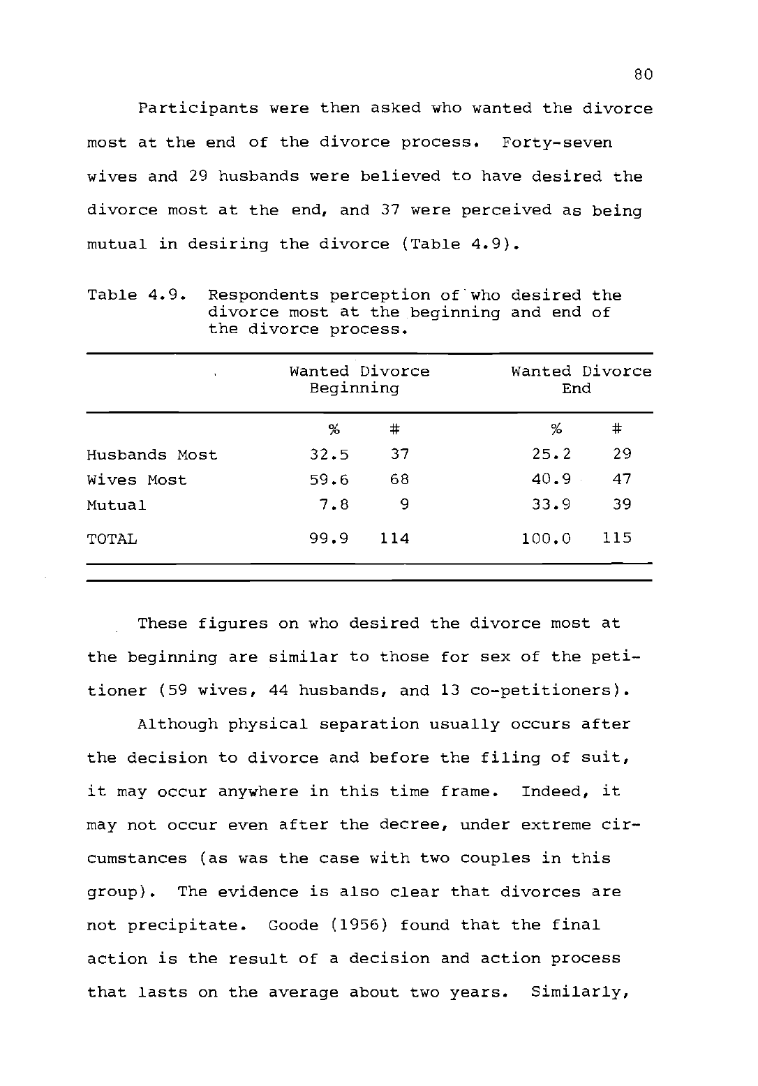
80
Participants were then asked who wanted the divorce
most at the end of the divorce process.
Forty-seven
wives and 29 husbands were believed to have desired the
divorce most at the end, and 37 were perceived as being
mutual in desiring the divorce (Table 4.9).
Table 4.9.
Respondents perception of who desired the
divorce most at the beginning and end of
the divorce process.
Wanted Divorce
Wanted Divorce
Beginning End
%
#
%
#
Husbands Most
32.5 37 25.2 29
Wives Most
59.6 68 40.9 47
Mutual
7.8 9 33.9 39
TOTAL 99.9 114
100.0
115
These figures on who desired the divorce most at
the beginning are similar to those for sex of the peti-
tioner (59 wives, 44 husbands, and 13 co-petitioners).
Although physical separation usually occurs after
the decision to divorce and before the filing of suit,
it may occur anywhere in this time frame. Indeed, it
may not occur even after the decree, under extreme cir-
cumstances (as was the case with two couples in this
group).
The evidence is also clear that divorces are
not precipitate.
Goode (1956) found that the final
action is the result of a decision and action process
that lasts on the average about two years. Similarly,

81
the average time of separation for the couples in this
group was 21 months, which meant that nearly two years
had elapsed between physical separation and the final
decree.
Also of note is the range of time which elapsed
between the decision to divorce and the final decree.
The minimum time period for obtaining a divorce in
Oregon is 90 days.
This statutory waiting period can
be waived by .a circuit court judge upon a showing of
hardship by either spouse.
This would account for the
minimum separation time of one month. Some couples
waited a number of years before formalizing their sep-
arate living arrangements, the maximum period of sep-
aration being over 15 years.
There are five major decisions where divorcing
couples may need to reach agreement:
child custody,
visitation, child support, spousal support and division
of property (Kressel, et al, 1978).
Respondents report-
ed that 56 couples made these decisions themselves.
Twenty-four respondents reported that decisions were
negotiated by attorneys.
Respondents reported that 20
couples brought their case to court, where the presiding
judge had the major responsibility for award decisions.
Only three respondents reported using a mediator or me-
diation process.
Even if the couples were making the decisions, it
was not without benefit of legal counsel.
Both partners

82
had their own attorney in 70 instances and in 17 cases
only one spouse was represented by an attorney.
Nine
couples used the same attorney, and 17 couples filed
their divorce papers themselves.
If the respondent indicated that the couple had
made the decisions about dividing property themselves,
they were asked a follow-up question, "When you were
making the decisions on how to divide things, do you
think your input related to those decisions, and the
input of your former spouse was equal, nearly equal,
neither equal nor unequal, more unequal than equal, or
unequal?" Of the 56 couples making their own decisions,
38 respondents indicated that their inputs were equal
or nearly equal. Nine respondents said that their in-
puts were either unequal to more unequal than equal.
Three participants indicated inputs were neither equal
nor unequal.
One woman said, "I knew as much as he did,
but he could talk faster than I could!"
Division of Property
It was expected that gender and duration of mar-
riage would affect the amounts and types of assets owned
and divided between wives and husbands.
One hundred one
cases involved home ownership. In 53 cases (52.4 per-
cent of the cases involving homes) the wife continued to
live in the family home.
In 27 cases (26.7 percent of
the cases involving homes) the husband continued to live

83
in the family home.
A few couples (6) retained joint
ownership in the home or sold the home immediately and
divided the proceeds (5.9 percent of the cases involving
homes).
However, the full equity in the home was not
always retained by the spouse who continued to live
there.
In 24 cases the wife stayed in the house and
the husband received a cash settlement to be paid over
time or when the house was sold.
In 17 cases the hus-
band continued to live in the house and the wife kept
her share of the equity.
Twenty-nine wives and ten
husbands retained the full value of the family home.
Table 4.10 presents the data regarding the ultimate
disposition of the family home.
Table 4.10. Disposition of family home.
(n)
To wife - full value
To wife
part value
28.7
23.8
29
24
To husband - full value 9.9
10
To husband
part value
16.8 17
Sell and divide or joint 5.9
6
No value determined
14.9 15
TOTAL
100.0
101
There were 37 couples who owned other real estate.
Of these couples, 18 husbands and seven wives retained
the other real property.
Eleven of the couples divided
the value.
In one instance the other real estate was

84
repossessed between physical separation and the final
decree.
All but two of the couples owned at least one car
prior to the divorce.
In 27 families, only one car was
owned.
In 16 of these families, the wife kept this
asset. In 11 cases, the husband kept the family car.
One couple decided the wife should keep their only
car since there was no public transportation from her
new residence to her place of work.
Her husband, who
had custody of the couple's three children, took the
children to and from day care and traveled to work on
the bus.
In families with two cars, equal division of
the cars was more likely.
If three cars were owned,
the husband usually kept two and the wife kept one. In
three instances, the couple owned between six and eight
cars and the husband kept all but one or two of them.
Of the 38 couples who owned other vehicles such as
a boat, camper, trailer, or motorcycle, wives retained
the other vehicle in only five instances.
In all other
cases (33) the husband kept the other vehicle(s).
House-
hold furnishings were kept by the wife in ten of the
cases in which a value was placed on them.
They were
fairly evenly divided in 23 of the cases where it was
specifically valued.
Bank accounts were divided between husband and wife
in 54 cases (51.4 percent) of the 105 couples who owned
this asset.

85
Thirty-seven couples owned stocks, bonds, or other in-
vestments.
Of these, 12 husbands and ten wives retained
ownership of these assets. Thirteen couples divided
those assets. One couple could not agree on how their
stock should be divided (the husband was a stockbroker).
When their case finally went to court, the judge arbi-
trarily picked four stocks (all blue chip in the percep-
tion of the wife who told this story) and awarded them
to the wife. .
Businesses or professional practices went predomi-
nately to husbands (23 out of 34 cases), but seven wives
retained this asset. One couple divided the family
business, with the wife taking enough equipment and in-
ventory to start again in another state. In three
cases, both spouses kept their own professional prac-
tices.
Ownership of pensions and retirement funds varied
greatly with gender, as well as with marital duration
and family income. Husbands were much more likely than
wives to have acquired pensions during marriage.
Mar-
ried women were much less likely to acquire pensions,
irrespective of the length of their marriage or age.
When both husband and wife had pensions, the husband's
pension was of much greater value.
In terms of frequen-
cy of ownership, pensions were the asset most often men-
tioned after furniture, cars, family home, and bank
account.
Husbands and wives were equally likely to keep

86
their own pensions in a divorce settlement.
Forty-two
of the husbands who had pensions kept the full amount
of their retirement benefits, as did six wives who had
pensions.
Three wives received a share of their hus-
band's pension.
In 28 cases where both husband and wife
each owned a pension, each spouse kept his/her own.
Forty-eight couples owned life insurance with a
cash value, such as a whole life policy.
Life insurance
policies were always kept by the titled owner.
The average amount of debt, excluding mortgages
and car loans, retained by husbands was $6,296.48
(median $2,400).
The average amount of these debts re-
tained by the wife was $1,870 (median $796.50).
Participants were asked to estimate the shares
they received of all the personal and real property and
their level of satisfaction with the division of prop-
erty.
About one-third of the female respondents and
one-third of the male respondents said they received
less than half the property in the settlements.
Eigh-
teen wives and 12 husbands reported receiving more than
half the property. Seventeen wives and 15 husbands re-
ported that their common holdings were divided on a
fifty-fifty basis.
Table 4.11 presents this data re-
garding their estimate of the division.

87
Table 4.11.
Estimate of division.
Husbands Wives
%
(n)
%
(n)
All
8.2 4 9.1
More than half
24.5 12 27.3
18
About half
30.6 15 25.8 17
Less than half
34.7 17 34.8 23
None
2.0 1 3.0 2
TOTAL
100.0 49 100.0
66
Whatever the division, 18 wives and 17 husbands
tended to be somewhat or very satisfied with it.
How-
ever, 16 wives and 11 husbands were somewhat or very
dissatisfied with their settlement. Twelve individuals
(seven wives and five husbands) stated that they were
neither satisfied nor dissatisfied with the property
division.
Table 4.12 summarizes their responses.
Table 4.12.
Level of
satisfaction with settlement.
Husbands Wives
% (n)
% (n)
Very satisfied 31.1 14 44.8
30
Somewhat satisfied 33.3
15 20.9 14
Neither satisfied nor
dissatisfied
11.1 5 10.4 7
Somewhat dissatisfied
11.1 5 6.0
4
Very dissatisfied
13.3 6 17.9
12
TOTAL
100.0
45 100.0 67

88
Spousal Support
The findings from this study would appear to sup-
port the conclusions of Weitzman (1979, 1981) and
McGraw, Sterin and Davis (1982) that relatively few
wives were granted spousal support and when support is
granted, recipients will receive it for a short peri-
od of time.
Women with custody of minor children and
women with fairly long marriage durations are the most
likely to receive spousal support (McGraw, Sterin and
Davis, 1982).
At the time these divorces were finalized,
ORS 107.105(1)(d) empowered the court, in a dissolution
case, to provide support "for such a period of time as
it may be just and equitable for the other party to con-
tribute."
In the leading case on spousal support in
Oregon, Grove v. Grove (1977), the Court of Appeals
stated that "The most significant factor (in ordering
spousal support) is whether the wife is employable at an
income not overly disproportionate from the standard of
living she enjoyed during the marriage.
The wife's em-
ployability includes consideration of her education,
training, experience, age, health, capacity, whether she
has custody of small children, etc."
In reaffirming
Grove, the Supreme Court added, "We will not ignore the
fact that, at least until recent years, young women en-
tering marriage were led to believe--if not expressly by
their husbands-to-be, certainly implicitly by the entire

89
culture in which they had come to maturity--that they
need not develop any special skills or abilities beyond
those necessary to homemaking and child care, because
their husbands, if they married, would provide their
financial support and security. We cannot hold that wo-
men who relied on that assurance, regardless of whether
they sacrificed any specific career plans of their own
when they married, must as a matter of principle be
limited to the standard of living they can provide for
themselves if 'employed at a job commensurate with
(their) skills and abilities.'
The marriage itself may
well have prevented the development of those skills and
abilities" (Grove v. Grove, 1977).
A comparison of Tables 4.8 with Table 4.14 supports
the conclusion that many of the wives in this sample are
living at much lower standards than they enjoyed during
marriage.
Yet only 32 wives had orders for spousal sup-
port. This relatively low proportion of support orders
suggests that there is an expectation of self-suffi-
ciency for most divorced women and a gap between the
law's stated intent to provide support for women with
impaired earning capacities and reality.
Two other items, duration and amount, complete this
summary of the pattern of support orders. Eighteen sup-
port orders were for a specified period ranging from
four to 144 months, with a mean of 38.9 months--just
over three years. Fourteen wives received "permanent"

90
support (for the lifetime of either spouse or until the
wife's remarriage). The amount of spousal support rang-
ed from $50 to $1350 a month, with a mean of $432.65
(median $400).
It should be noted that five of these
awards called for the amount of support to be "stepped
down" over the period for which it was granted. In no
instance was spousal support tied to a cost of living
increase or increases in the obligor's salary. Twelve
wives received a property judgement (other than family
home equity) which may be paid in periodic installments
similar to spousal support, and six of these 12 women
received spousal support as well. At the time the
interview was conducted, (25) respondents from the group
where spousal support was ordered reported paying or re-
ceiving the full amount every month.
(Note: Oregon's spousal support laws are sex-
neutral, either party may be obligated for support, but
out of the 566 couples in the entire sample, only one
husband was given spousal support, and that only until
the family restaurant was sold. Neither husband nor
wife could be interviewed.)
Decisions Pertaining to Children
Three major decisions pertaining to children are
found in divorce decrees: custody, visitation, and the
amount of child support. The key finding relative to
custody was that mothers continued to have custody of

91
some minor children in the majority of cases (66 of the
85 cases involving children). Split or joint custody
was the arrangement in 25 of the cases involving child-
ren. Sharing parental responsibility took many legal
forms.
Sometimes, joint custody meant joint legal and
physical custody; in some cases, one parent was desig-
nated as the primary physical custodian; some couples
separated the children so both parents had children in
their custody.
There has been a small, but meaningful,
change in terms of fathers who have custody.
In this
sample, 20 fathers had custody of some minor children.
(These totals add to more than 85 because of the number
of cases involving split custody.)
Child support was required almost entirely of
fathers:
in only six cases was a mother required to pay
support, and, in two cases, both parents were required
to pay support. When the mother is the custodial par-
ent, she is more likely to be awarded child support from
the noncustodial parent (62 cases of the 85 cases involv-
ing children) than when the father is custodial parent.
More frequently, when the father has custody, neither
parent is obligated for child support payments.
In
seven cases involving split custody, the father was also
making child support payments to the mother.
The amount
of child support ranged from $25 to $667 a month, for an
average of $209.49 a month (median $188.50).
Only two
of these orders involved an increase in the amount of
92
support over time. One mother would receive a raise in
child support after the father had been in practice for
three years. Another increase was tied proportionally
to the father's increases in salary.
The incidence of arrears for child support, nation-
ally, is reported to be very high--especially as time
after the decree increases (Eckhardt, 1968).
In 1981,
only 47 percent of the custodial parents with child
support orders received the full amount due (Child
Support and Alimony, 1983).
In this sample group, 72
cases involved orders for child support.
Fifty-two
parents reported paying or receiving the full amount
every month.
Fourteen (parents) reported paying or re-
ceiving child support "sometimes" or "rarely" and six
parents reported never paying or receiving child support.
Several explanations may be possible for this high com-
pliance rate: relatively little time may have elapsed
between the final decree and the interview, interviewed
obligors may be giving "socially acceptable" answers,
and, the duration of marriage is longer and parents'
ages older for this group than a random sample of all
divorces, which could result in higher incomes and a
longer period of emotional attachment to dependent chil-
dren (Luck, 1985).
Interestingly, when fathers are or-
dered to pay child support, 73.8 percent of the parents
reported paying or receiving the full amount regularly
every month.
Of the six mothers obligated to pay child

93
support, two were in full compliance, two paid support
"sometimes" and two had never paid support.
In Oregon, divorce decrees commonly include pro-
visions governing child support payments and the non-
custodial parent's visitation with the child(ren).
Some couples preferred elaborate stipulations as to
visitation--so many days per week or per month, specific
holidays or vacations, sometimes specifications of birth-
days and excluded times. The most common visitation
provisions are "reasonable and seasonable," relying on
the parents to cooperate to make visitation work effec-
tively. In the rare instance where visitation was lim-
ited, court records contained evidence of alcohol, drug
or sexual abuse by the visiting parent.
Although child support and visitation should be
two separate issues, parents with custody of children
sometimes refuse visitation rights to the parent paying
support when support payments fail behind. By the same
token, withholding support could be employed when the
paying parent felt visitation rights were being refused.
A recent report by the Governor's Commission on Child
Support Enforcement recommended that, as a policy,
visitation rights should be enforced with the same vigor
as enforcement of child support.
"Failure to comply
with an order in either of these areas should not be an
acceptable reason for failure to comply with the order
in the other area" (Governor's Commission on Child Sup-

94
port Enforcement, 1985).
Economic Well-Being After Divorce
Participants were asked to compare their present
economic situation with their pre-divorce economic sit-
uation.
Here, opinion was sharply divided between wives
and husbands.
Fourteen husbands and 14 wives believed
their present economic situations were better.
Thir-
teen wives and 1.1 husbands said their economic situa-
tions were about the same.
However, 22 wives believed
their present economic situations were worse, compared
to ten husbands.
Several respondents, while admitting
that their actual income from all sources was less than
during the marriage, said control over their present in-
come was the overriding factor.
"I don't have to be
responsible for his gambling debts any longer," or "She
can't run up my charge accounts now."
One husband re-
plied laconically, "There's one less mouth to feed."
Table 4.13 summarizes their responses.

95
Table 4.13.
Attitude toward present economic situation.
Husbands Wives
% (n)
% (n)
Better
28.6 14 20.9 14
Somewhat better
10.2 5 10.4 7
About the same 22.4 11 19.4 13
Somewhat worse 16.3 8 16.4 11
Worse
20.4 10 32.8 22
Don't know
2.0 1
.0 0
TOTAL 100.0 49 100.0 67
Earlier, the annual household incomes prior to
divorce were presented, as well as the monthly incomes
of wives and husbands at the time of the divorce. The
following table compares household income for wives and
husbands following the divorce. Two sets of income
transfers have been taken into account in these figures.
Child and/or spousal support payments have been added
to respondent's income when the respondent indicated
that it was being paid.
Likewise, child and/or spousal
support payments have been deducted from income of re-
spondent when the respondent indicated it was being
paid. If respondent had remarried, income from the new
spouse was also included, as was any income received
from a domestic associate.

96
Table 4.14.
Present household income of respondents.
Husbands
Wives
%
(n)
% (n)
Less than $5,000 2.0
1
10.4 7
$5,000 to $9,999
4.1 2 10.4 7
$10,000 to $14,999
4.1 2
22.4 15
$15,000 to $19,999
14.3 7 11.9
8
$20,000 to $24,999
14.3 7 14.9 10
$25,000 to $29,999
12.2
6 10.4
7
$30,000 to $39,999 22.4 11 11.9 8
$40,000 to $49,999 6.1 3 3.0 2
$50,000 or more 20.4 10 4.5 3
TOTAL 100.0 49
100.0 67
When respondents were asked about the largest
source of their income at the time of the interview,
earned income was the largest source of 42 wives and 43
husbands.
Of note is the fact that no husbands reported
the largest source of their present income to be salary
from a new spouse (or domestic associate) or from ali-
mony/child support, although 16 wives reported these as
the largest source. Table 4.15 summarizes their present
income sources.

97
Table 4.15.
Largest source of present income.
Husbands Wives
% (n)
% (n)
Earned salary 89.6 43
64.6 42
Remarriage .0 0 12.3
8
Welfare/unemployment 2.1 1
4.6
3
Retirement/Social Security 2.1 1
4.6
3
Alimony/child support
.0
0
12.3
8
Investments/business
6.3 3 1.5
1
TOTAL 100.0 48 100.0
65
There was one question to which nearly all par-
ticipants had the same answer. When asked to compare
their present emotional situation with that during the
marriage, overwhelmingly the answer was "Better, Better,
Better!" When asked "Why," one wife responded, "How
much time do you have?"
Table 4.16.
Attitude toward emotional situation.
Husbands
Wives
%
(n) % (n)
Better
83.7 41 71.2 47
Somewhat better
4.1 2 18.2 12
About the same
4.1 2 3.0 2
Somewhat worse
4.1 2
3.0
2
Worse
4.1 2
4.5 3
TOTAL 100.0 49 100.0 66

98
Hypothesis Testing
All hypotheses have been stated in the null form
for the purpose of statistical analysis.
Ownership of Assets
It was hypothesized (H01) that there would be no
relationship between the types of assets owned by di-
vorcing couples and the parties' ages, employment his-
tories, monthly incomes, education levels, duration of
marriage, and number and ages of dependent children.
For the purpose of this study, each asset was placed in-
to one of these four categories:
family home, other
real property, tangible personal property (e.g., cars,
other vehicles, furniture, and household durables), and
intangible personal property (e.g., bank accounts, stocks
and bonds, pension and retirement benefits, life insur-
ance, and business or professional practices).
After utilizing the Student's t-test it was found
that no significant differences existed between owning
a family home and husband's age, wife's age, years mar-
ried, children's ages, number of minor children, hus-
band's length of employment, and wife's length of em-
ployment. In X2 analyses cross tabulating the relation-
ship between owning a family home and husband's income,
wife's income, husband's level of education, and wife's
level of education, no significant relationships were

99
found.
A t-test analysis was utilized to find if there was
a significant relationship between ownership of other
real property and wife's age, husband's age, years mar-
ried, number of minor children, children's ages, hus-
band's length of employment, and wife's length of em-
ployment.
A significant relationship was found by this
analysis between the number of minor children and owner-
ship of other real property (t-value = -2.12, p= .036)
(Table 4.17). People who owned real estate other than
a family home had fewer children than those who did not
own other real property.
Table 4.17. Number of minor children for those who
owned other real property and those who
did not own other real property.
Mean S.D.
Owned other real property
1.1081 .994
Did not own other real property 1.5584
1.094
Two-tailed t-test, t-value = -2.12, p= .036
In X
2
analyses cross tabulating ownership of other
real property with husband's income, wife's income, hus-
band's education level, and wife's education level, no
significant relationships were found.
A t-test analysis of respondents who owned tangible
personal property and those who did not own tangible

100
personal property, by wife's age, husband's age, years
married, number and ages of minor children, husband's
employment history, and wife's employment history, found
no significant differences.
The reason for this may lie
in the definition of tangible personal property.
Inclu-
sion in this category was determined by whether the re-
spondent owned any of the following:
household furni-
ture and durables, cars, and other vehicles. All of the
respondents owned furniture, and 114 owned cars, so no
valid comparisons could be made as there were no couples
who did not own at least one of the items of tangible
personal property.
Further analysis consisted of X
2
cross tabulations
comparing the relationship between ownership of tangible
personal property and husband's income, wife's income,
husband's education level, and wife's education level.
Again, no significant relationships were found, because
there were no couples who did not own some tangible per-
sonal property.
In comparing those respondents who owned intangible
personal property with those who did not by wife's age,
husband's age, years married, number and ages of minor
children, and husband's employment history, no signifi-
cant differences were found.
There was a significant
difference between the two groups by wife's employment
history (t-value = 2.46, p= .016) (Table 4.18).
The
longer period of time the wife was in the paid labor

101
force, the more likely the couple was to have owned one
of the items defined as intangible personal property:
bank accounts, stocks and bonds, pension and retirement
benefits, life insurance, and businesses or professional
practices.
One explanation for this finding may be that
the longer the wife is employed, the more her income
increases, and there would be more disposable income for
investing in these assets.
However, when wife's income
and ownership of intangible personal property were anal-
yzed, no significant relationship could be found (X
2
=
10.37, p= .240).
Another explanation of this relation-
ship is the number of wives who have accumulated pension
benefits through employment.
Caution should be exer-
cised in interpretation of these results, however, be-
cause of the small number of couples who did not own at
least one item of intangible personal property.
Table 4.18. Ownership of intangible personal property
by wife's employment history.
Mean
Owned intangible 9.556
(n= 106)
Did not own intangible
1.333
(n= 3)
Two-tailed t-test, t-value = 2.46, p= .016
S.D.
5.764
1.528
Further examination of intangible personal prop-
erty ownership by husband's income, wife's income, and

102
husband's education level found that no significant re-
lationships existed.
However, ownership of intangible
personal property and wife's education level was found
to be highly significant
(X2
= 40.84, p= .000) (Table
4.19).
Table 4.19. Ownership of intangible personal property
by wife's education level.
Owned Did Not
Intangible
Own
% (n) % (n)
Grade school
1.8 2 .0
0
Some high school 2.7
3
75.0
3
High school graduate
22.7 25
.0
0
Trade school/beyond
high school 7.3
8 .0
0
Some college 38.2
42 25.0 1
College graduate
14.5 16
.0
0
Some graduate work
.9 1
.0
0
Graduate degree
11.8
3 .0 0
TOTAL
100.0 110 100.0
4
X
2
= 40.845, p= .000
This relationship may be spurious, however, because
of the small number of cases in group two, those who did
not own intangible personal property.
Hol could be re-
jected based on the data collected for this study.
Dollar Value of Assets
In this study, it was hypothesized (H02) that there

103
would be no difference between the dollar value of
assets owned by divorcing couples and the parties' ages,
their employment histories, their monthly incomes at the
time of divorce, education levels, marital duration, and
the number and ages of their minor children. A new vari-
able, assets minus debts (ASMD), was created by summing
the equities in eleven assets: family home, other real
property, cars, other vehicles, furniture, bank ac-
counts, stocks and bonds, business or professional prac-
tice, insurance, pensions, and any other asset which did
not fall into one of the other categories of property.
To this total was added the value of any property judge-
ment (other than family home equity). From this sum of
assets, the amount of debts assumed by both husband and
wife was subtracted to arrive at a net dollar value of
assets for each family interviewed. Assets minus debts
could only be computed for 76 individuals because, in
many instances, either the wife's debt or the husband's
debt, or both, were missing.
A correlation matrix based on Pearson's Product
Moment correlation coefficient was established to ascer-
tain the significance of relationships between selected
characteristics of the couples and the net dollar value
of assets.
Significant relationships were found to
exist between the net dollar value of assets and wife's
age (p= .007), husband's age (p= .015), years married
(p= .005), number of minor children (p= .009), and the

104
amount of child support ordered per child per month
(p= .001) (Table 4.20).
No significant relationship
was found between net dollar value of assets and the
employment histories of husband or wife, ages of minor
children, number of children in either parent's custody,
and the duration and amount of spousal support ordered.
As might be expected, the amount and value of
assets increased with marital duration and the parties'
ages.
The net dollar value of assets also increased
with the number of minor children.
The family home was
the most variable asset for most couples.
Housing be-
havior is likely to be governed by the age, spacing,
sex and number of children (Morris and Winter, 1978).
It was also expected that the amount and value of
assets would increase with family income.
Yet, no sig-
nificant relationships were found between the net dollar
value of assets and wife's income, husband's income,
wife's education level, or husband's education level.
What is even more puzzling about these findings is that
there is partial support for a difference in net dollar
value of assets and income, in that ASMD is positively
correlated with the amount of child support ordered per
child per month.
Higher amounts of child support were
accompanied by an increase in net dollar value of
assets.
In Oregon, an order for payment of child sup-
port is based upon the premise that both parents are
obligated to support their children within their capac-
105
ity to do so.
There is no precise formula for determin-
ing the amount of child support which a parent will be
ordered to pay in any particular case. Smith v. Smith
is case law in relation to determining the proportion
of support that each parent will be required to provide,
and that proportion is based on the incomes of both par-
ents and the needs of the child. Based on the data col-
lected for this study, H02 was rejected.

Table
4.20.
Correlations between selected characteristics
the net dollar value of assets.
of divorcing
couples and
ASMD WAGE
HAGE YRMR
WYE HYE
NMCHD CHAV
NWCDY
NHCDY PCPM
SPPM DSP
WAGE
RAGE
YRMR
WYE
HYE
NMCHD
CGAVG
NWCDY
NHCDY
PCPM
SPPM
DSP
.007*
.015*
.005*
.773
.112
.009*
.125
.558
.264
.001*
.064
.277
.001
.001
.006
.001
.001
.001
.595
.704
.186
.394
.001
.001
.093
.001
.001
.001
.631
.370
.489
.526
.002
.009
.001
.001
.001
.583
.577
.178
.004
.023
.070
.002
.110
.628
.188
-.897
.587
.803
.010
.001
.605
.435
.688
.007
.089
.036
.001
.137
.214
.609
.043
.084
.172
.925
.643
.637
.001
.071
.316
.036
.036
.081
.543
.001
.648
.870
107
Valuation of Assets
One of the surprising findings from the pilot study
conducted in Benton County in 1983 was the infrequent
mention of property values in court records. Only the
handful of cases that went to court included dollar
values.
Then there were three values listed:
the pe-
titioner's, the respondent's, and the judge's. Debts
were reported in many cases, but outstanding mortgages
only occasionally.
This was also true of this sample,
although there appeared to be somewhat more data in the
court records. When the couple made the decisions as
to asset allocation, or when the settlement was negoti-
ated by attorneys, financial reporting was almost nil.
The face-to-face interviews permitted a determination
of just how the values of property which divorcing cou-
ples were dividing was established. For the purpose of
this study, two methods of valuation were defined:
ob-
jective (if some data such as an independent appraisal,
property tax records, Blue Book, classified advertise-
ments, retirement account statements, or bank state-
ments were used); or subjective (if no data were used
to arrive at a fair market value). Although Oregon law
does not mandate an equal division of property, only
one which is "just and proper in all the circumstances,"
courts strive to give each spouse an equal share in the
assets when the marriage has lasted for ten years or

108
more (Gildea, 1981, Graham, 1983).
It began to appear,
after the pilot test, that subjectively valued assets
were being used to balance the scale between husband
and wife, regardless of the actual value of the asset.
Furthermore, it appeared that the bulk of subjectively
valued assets was being kept by wives.
So it was hypothesized (H03) that there would be
no difference between how assets are valued for divi-
sion and who retained the asset.
Eleven X
2
statistical
analyses were utilized.
No significant relationships
were found.
H
o
3 could not be rejected.
There were no
differences between how assets were valued for division
and who retained the asset.
Table 4.21 summarizes the
methods of valuation used by divorcing couples by asset
categories.

Table 4.21.
Method of
couples.
109
asset valuation used by divorcing
# of
No Spe-
cific
Couples Objective], Subjective
Value Re-
Asset Owning Valuation
Valuation
ported
Family
home 101 58.4 59
11.9 12 29.7 30
Other real
property
37
51.3 19 24.3 9 24.3 9
Cars
114
31.5 36 29.8 34 38.6 44
Other
vehicles
38 23.6 9 23.6 9 52.6 20
Furniture 116 7.7
9 20.7 24 71.6 83
Bank
account 105 56.1
59
7.6
8 36.2 38
Stocks/
bonds 37 59.4 22 5.4
2 35.1 13
Business/
practices
34 44.1
15 26.5 9 29.4 10
Insurance 48 43.7 21 10.4 5 45.8 22
Pension 76
30.2 23 7.9 6 61.9 47
Any other
asset 30 53.3 16 23.3
7
23.3 7
1
Assets were considered objectively valued if some data
(i.e., independent appraisal, property tax records,
Blue Book, classified advertisements, retirement
account statement, bank statements) were used to
determine fair market value.
2
Assets were considered subjectively valued if no data
were used to determine fair market value.

110
There was an indication, from participants' an-
swers, that there is a great deal of "separateness" in
marital property concepts.
For example, "Well, it was
his mother's furniture, so he took it," or "We both had
pensions, so I kept mine and she kept hers."
Oregon is
an equitable distribution state which considers all the
"real and personal property, or both, or either or both
of the parties" for division at dissolution, regardless
of when or how acquired (ORS 107.105(f)).
No distinc-
tion is made between "marital property" and "separate
property."
Perhaps what is being seen is the emergence
of individual concerns in the context of marital disso-
lution.
The "we" dream is over, and the "yours or mine"
reality is beginning (Prager, 1977).
Allocation of Assets
Over a ten year period in California, Weitzman
(1981) found that "wives remain more likely to be award-
ed the family home and household furnishings, while hus-
bands are usually granted other real estate, the busi-
ness, and the family car."
Researchers in Ohio (McGraw,
Sterin and Davis, 1982) discovered that "businesses and
real estate usually go to the husband and furniture usu-
ally was awarded to wives."
It was hypothesized (H04)
that there would be no difference in the types of assets
allocated to wives and allocated to husbands by the par-
ties' ages, their employment histories, their monthly

111
incomes, their education levels, number of children in
each parent's custody, amount of child support ordered,
amount and duration of spousal support ordered, who
wanted the divorce most in the beginning and at the end
of the divorce process, whether or not the couple had
made the decisions about asset allocation, and the net
dollar value of the couple's assets. The four types of
property analyzed were:
family home, other real prop-
erty, tangible personal property, and intangible person-
al property.
Analyses of variance found no difference in which
spouse kept the family home by wife's age, husband's
age, years married, wife's employment history, husband's
employment history, amount of child support ordered per
child per month, amount and duration of spousal support,
or the net dollar value of assets.
However, custody de-
cisions did have a significant effect. Both wives (F=
4.155, p= .0211) (Table 4.22) and husbands (F= 5.210,
p= .0110) (Table 4.23) who kept the family home had
custody of more children than wives or husbands who did
not keep the family home or in situations where the fam-
ily home was kept in joint ownership or sold and the
proceeds divided. These findings were consistent with
those of Ohio researchers who found custodial fathers
and custodial mothers received a larger share of the
marital home, 80 percent and 70 percent, respectively
(McGraw, Sterin and Davis, 1982).

112
Table 4.22.
Wives keeping family home by custody of
children.
Source
Sum of
Mean
Squares
DF Squares
Ratio Prob.
Between Groups
6.4676 2
3.2338 4.155
.0211
Within Groups 41.2467
53 .7782
Total
47.7143
55
F*=4.155, with 2.53 d.f., do not reject at the .05 level
of significance
Table 4.23.
Husbands keeping family home by custody of
children.
Source
Sum of
Mean
Squares DF
Squares Ratio
Prob.
Between Groups
6.5270
2 3.2635
5.210 .0110
Within Groups
20.0444
32 .6264
Total
26.5714 34
F*=5.210, with 2.32 d.f., do not reject at the .05 level
of significance.
In X
2
analyses cross tabulating sex of spouse keep-
ing the family home and wife's income, husband's income,
who wanted the divorce most at the beginning and end of
the divorce process, wife's education, husband's educa-
tion, and whether the couple had made the decisions as
to asset allocation, no significant differences were
found.
Comparison of who retained real property other than
the family home by husband's age, wife's employment his-

113
tory, number of children with each parent, amount of
child support ordered per child per month, amount and
duration of spousal support, and net dollar value of
assets found no significant differences.
It was found
that wife's age, years married, and husband's employ-
ment history did make a significant difference.
Wives
who kept other real property were younger (F = 3.298,
p = .0498) (Table 4.24) than wives whose husbands kept
the other real estate or wives who divided the value of
other real property with their former spouses.
Table 4.24. Retention of other real property by wife's
age.
Source
Sum Mean
Squares DF Squares Ratio Prob.
Between Groups 634.5984 2 317.2992 3.298 .0498
Within Groups 3078.5444 32 96.2045
Total 3713.1429 34
F*=3.298, with 2.32 d.f., do not reject at the .05 level
of significance
It was also found that husbands who divided the
value of other real property with their former spouses
were married longer (21.4 years) than husbands who re-
tained the full value of other real estate (16.2 years)
or husbands whose wives received the other real property
(F = 3.314, p = .0488) (Table 4.25).

114
Table 4.25. Retention of other real property by marital
duration.
Source
Sum of
Mean
Squares DF Squares Ratio Prob.
Between Groups
255.7053
2 127.8526 3.314
.0488
Within Groups 1273.2670 33 38.5838
Total 1528.9723 35
F*=3.134, with 2.33 d.f., do not reject at the .05 level
of significance
Although wife's employment history had no signifi-
cant effect on retention of other real property, hus-
band's employment history did. Husbands who divided the
value of other real property with their wives were em-
ployed longer (20.9 years) than husbands who retained
other real property (14.7 years) or husbands whose wives
kept other real property (14.0 years) (F = 3.186, p =
.0543) (Table 4.26).
Table 4.26. Retention of other real property by
husband's employment history.
Source
Sum of
Mean
Squares DF Squares Ratio Prob.
Between Groups
314.4520 2 157.2260
3.186 .0543
Within Groups
1628.5202 33 49.3491
Total
1942.9722 35
F*=3.186, with 2.33 d.f., do not reject at the .05 level
of significance

115
To determine if there were differences in the reten-
tion of tangible personal property, analyses of variance
were utilized.
No significant differences were found by
wife's age, husband's age, years married, wife's employ-
ment history, husband's employment history, number of
children with husband, amount of child support ordered
per child per month, amount and duration of spousal sup-
port, or net dollar value of assets. A significant dif-
ference did exist between retention of tangible personal
property and the number of children with the wife. Wives
whose husbands retained most or all of the couple's
tangible personal property (furniture and household dur-
ables, cars, and other vehicles) had custody of fewer
children (.250) than wives who divided these assets with
their former spouse (1.626) or wives who retained most
or all of the couple's tangible personal property (2.00)
(F = 5.064, p = .0087) (Table 4.27). It seems reasonable
that the parent having custody should retain the mari-
tal home and furniture, allowing the children to remain
in their customary environment.

116
Table 4.27.
Retention of tangible personal property by
children's custody.
Source
Sum of Mean
Squares DF Squares
Ratio Prob.
Between Groups 8.1047 2 4.0523 5.064 .0087
Within Groups 58.4216 73 .8003
Total 66.5263
75
F*=5.064, with 2.73 d.f., do not reject at the .05 level
of significance
When retention of tangible personal property was
compared with husband's income, who wanted the divorce
most at the beginning of the divorce process, wife's
education level, husband's education level, and whether
the couple had made the decisions as to asset allocation;
no significant differences were found.
A significant
relationship was found between retention of tangible
personal property and wife's income (X
2
= 26.856, p =
.020), showing that wives in the three lowest income
categories ($300 to $599 a month, $600 to $899 a month,
and $900 to $1,099 a month) were more likely to retain
most or all of the couple's tangible personal property
than wives in higher income categories. However, five
income cells were empty as couples had more of a tendency
to divide these assets at all other income levels.
Who
wanted the divorce most at the end of the divorce pro-
cess was also found to make a significant difference.
Wives were more likely (X2 = 9.98, p = .025) (Table 4.28)

117
to keep most or all of the couple's tangible personal
property when they wanted the divorce more than the hus-
band at the end of the divorce process.
What may be in-
fluential here is the nonmutuality of the decision to
divorce. Kressel (1978) noted that noninitiators exper-
ience such diminished feelings of self-worth that the
ability to bargain constructively is inhibited.
Table 4.28.
Retention of tangible personal property by
who wanted divorce most at the end.
Wife Most
Husband
Most Mutual
% (n)
%
(n)
%
(n)
Husband Kept
2.04 1 1.26 0 1.70 4
Wife Kept
3.27 6 7.02 2 2.71 0
Divided
41.69 40 27.72 27
34.59 35
(n = 115)
X
2
value = 9.98, d.f. = 4; p = .025
No significant differences were found in the reten-
tion of intangible personal property (bank accounts,
stocks and bonds, pension and retirement benefits, life
insurance, and businesses or professional practices) by
wife's age, husband's age, years married, wife's employ-
ment history, husband's employment history, number of
children with either parent, amount of child support
ordered per child per month, amount and duration of
spousal support, net dollar value of assets, wife's in-

118
come, husband's income, who wanted the divorce most at
the beginning and end of the divorce process, wife's
education level, husband's education level, and whe-
ther or not the couple had made the decisions as to
asset allocation.
Hypothesis four was rejected based
on the data collected for this study.
Equitable Distribution
Equitable distribution is allocating property
upon divorce based upon the concept that marriage is a
partnership or shared enterprise (Rothman v. Rothman,
(1974).
At the heart of this concept is the realization
that both spouses contribute to the economic circumstan-
ces of a marriage, whether directly by employment or in-
directly by providing homemaker services (Golden, 1983).
Most states, including Oregon, have not embraced a fixed
rule of division (e.g., 50-50) but vest wide discretion
in the judge to achieve individualized justice.
Oregon
statutes provide little guidance for the court; case law
speaks only to "ensuring that the parties separate on as
equal a basis as possible under the circumstances"
(Glatt v. Glatt, 1979).
For the purpose of this study
then, a division of assets was considered equitable when
either party received no more than sixty percent or no
less than forty percent of the fair market value of all
assets.
Further, it was hypothesized (H05) that there
would be no relationship between equitable distribution

119
and the parties' ages, their employment histories, their
monthly incomes at the time of divorce, their employment
histories, their education levels, marital duration, the
number of children with each parent, amount of child
support ordered, the amount and duration of spousal sup-
port, who wanted the divorce most at the beginning and
end of the divorce process, whether or not the couple
made the decisions regarding asset allocation, net dol-
lar value of assets, and whether any of the four types
of assets were owned.
To determine equitability of asset allocation, a
new variable, percentage of assets to wife (PAW) was
created by summing the wife's retained equity in eleven
assets and adding the amount of any property judgement
she received other than family home equity.
Debts as-
sumed by the wife were then subtracted to create a net
asset value for each wife.
A percentage of the wife's
net assets was calculated in relation to the net dollar
value of all the couple's assets.
Percentage of assets
to wife could only be computed for 76 individuals be-
cause, in many instances, either the amount of husband's
debts, wife's debts, or both were missing.
The average
percentage of the couple's net assets retained by the
wife was 64.5 percent with a range of -$200 to $1320
(median 48.7 percent).
A frequency distribution of per-
centage of assets to wife is given in Table 4.29.
The
category labeled "-0 to 0" means the debts the wife
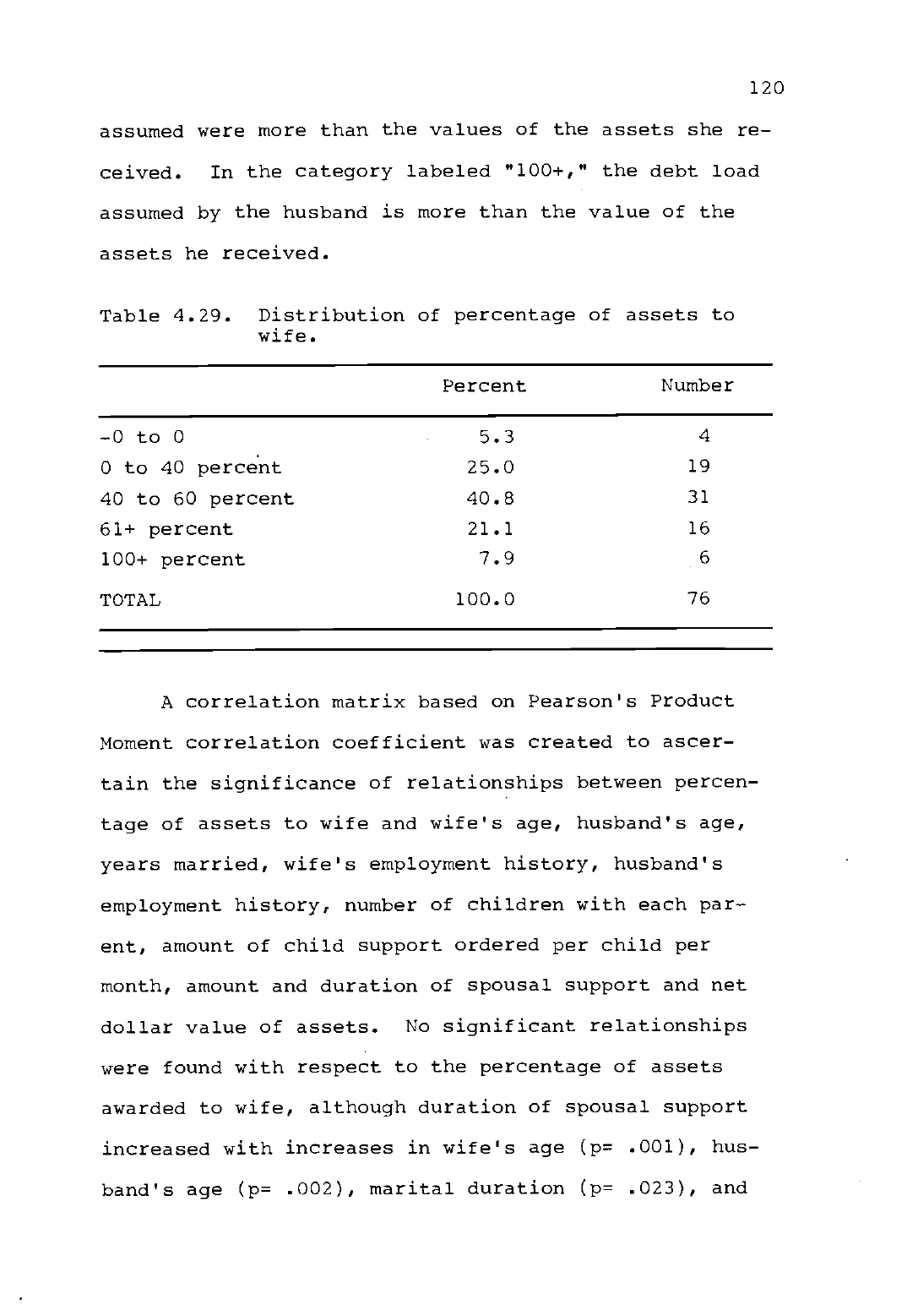
120
assumed were more than the values of the assets she re-
ceived.
In the category labeled "100+," the debt load
assumed by the husband is more than the value of the
assets he received.
Table 4.29.
Distribution of percentage of assets to
wife.
Percent
Number
-0 to 0
5.3
4
0 to 40 percent
25.0
19
40 to 60 percent
40.8
31
61+ percent
21.1
16
100+ percent
7.9
6
TOTAL
100.0 76
A correlation matrix based on Pearson's Product
Moment correlation coefficient was created to ascer-
tain the significance of relationships between percen-
tage of assets to wife and wife's age, husband's age,
years married, wife's employment history, husband's
employment history, number of children with each par-
ent, amount of child support ordered per child per
month, amount and duration of spousal support and net
dollar value of assets.
No significant relationships
were found with respect to the percentage of assets
awarded to wife, although duration of spousal support
increased with increases in wife's age (p= .001), hus-
band's age (p= .002), marital duration (p= .023), and

121
the number of children with wife (p= .036).
Further analyses did not find any significant rela-
tionships between percentage of assets to wife by wife's
income, husband's income, who wanted the divorce most at
the beginning and end of the divorce process, wife's
education level, husband's education level, whether or
not the couple made the decisions as to asset alloca-
tion, or by whether other real property, tangible per-
sonal property or intangible personal property was owned.
What was significant was the percentage of assets to
wife when a family home was owned (F= 4.946, p= .0293)
(Table 4.30).
When the couple owned a family home, the
wife received about half of the couple's net assets
(49.5 percent), but when a family home was not owned,
the wife received 163.5 percent of the couple's net
assets.
Since the family home is likely to be the most
valuable asset owned by middle-income families, this
suggests that when the wife receives the "long half,"
neither a family home nor any other asset of major value
was available for division.
Examination of the dollar value of assets retained
by wives and total dollar value of assets retained by
husbands, without subtracting debts, showed that hus-
bands received the larger dollar value of assets in 57
cases, wives received the larger dollar value in 55
cases, and four couples divided their assets absolutely
evenly.
To describe the typical division of property,

122
the median value is probably a better index because the
mean is more strongly influenced by a few high values.
Thus, the median division of assets is $33,635 to wives;
$30,511 to husbands. When debts are subtracted, the
median net value of assets to wives is $28,850; $24,908
to husbands. On the basis of data collected for this
study, H05 was rejected.
Table 4.30.
Percentage of assets to wife by ownership
Of family home.
Source
Sum of
Mean
Squares DF Squares Ratio Prob.
Between
112235.1489 2 112235.1489 4.946 .0293
Groups
Within 1633807.5818 72 22691.7720
Groups
TOTAL 1746042.7307 74
F*= 4.946 with 2.72 d.f., do not reject at .05 level of
significance
Post-divorce Economic Well-Being
Other researchers have found that no-fault divorce
laws have turned out to be "an economic disaster for
divorced women and minor children" (Weitzman, 1985).
In Ohio, McGraw, Sterin and Davis (1982) found that 1)
after termination of marriage, most husbands retain a
relatively high proportion of their former income--even
after all child support and/or spousal support orders
are paid, 2) there is an uneven relationship between

123
husband's and wife's post-divorce income--even if all
wives are employed and all income transfers are paid,
3) although both parties are affected financially in the
short term, divorce places an unequitable financial bur-
den on employed mothers and their children, and 4) moth-
ers who are not employed after divorce can expect to re-
ceive about one-fifth of their former income regardless
of the amount of their former family income. The Ohio
study concluded that there are much greater expectations
placed upon women in terms of financially supporting
themselves and their children after divorce.
Based on the results of these studies, the follow-
ing hypothesis (H06) was formulated: The post-divorce
economic well-being of wives and husbands has no rela-
tionship to the age of the respondent, years married,
respondent's employment history, household income prior
to divorce, number of minor children with respondent,
amount of child support paid or received by respondent,
amount of spousal support paid or received by respon-
dent, if respondent wanted the divorce most at the be-
ginning or end of the divorce process, education level
of the respondent, whether or not the couple made the
decisions as to asset allocation, the net dollar value
of assets received by respondent, sex of respondent, if
respondent was presently employed, and respondent's pre-
sent household income.
The stepwise multiple regression procedure avail-

124
able on the Honeywell Regress Subsystem (SIPS) was used
for this analysis.
At each step, the variable added to
the model is that one which makes the greatest contri-
bution to the reduction of the residual variability
below that achieved by the current model.
It will also
be the variable whose residual values have the highest
partial correlation with the residual values of the de-
pendent variable.
For the purpose of this study, post-divorce eco-
nomic well-being was determined by the respondent's
answer to Question 44:
"Do you think your economic
situation now, as compared to before the divorce is
better, somewhat better, about the same, somewhat worse,
or worse?"
Those independent variables entered into the
model, in order, were: 1) present employment of respon-
dent, 2) respondent's age, 3) marital duration, 4) whe-
ther or not the couple made the decisions as to asset
allocation, 5) net assets received by respondent, 6)
child support paid or received by respondent, 7) respon-
dent's education, 8) amount of spousal support paid or
received by respondent, and 9) respondent's sex. The
results of the regression analysis are detailed in Table
4.31.

125
Table 4.31.
Multiple stepwise regression of selected
variables on post-divorce economic
well-being.
Term entered
Beta
Entering
F p-value r
r
2
Respondent
presently
employed
1.13276
4.5636
.0369* .2701 .0729
Respondent's
age
-.145214
1.7874 .1866
.3179 .1011
Years
married .176300
6.4553 .0139*
.4404 .1940
Couple-
decisions .559418 3.0019 .0888
.4854 .2357
Respondent's
assets .113108 1.7098 .1966
.5091 .2592
Child
support
-.640303 2.3251 .1333 .5387
.2903
Respondent's
education
.882152 1.3874 .2395 .6301
.3971
Spousal
support
-.671463
.7953
.3771 .6361
.4074
Respondent's
sex .245356 1.4373
.2369 .6524
.4257
(n = 60)
Total explained variance by the group of indepen-
dent variables is .42.
The nine independent variables
explained 42 percent of the respondent's attitude to-
ward their present economic situation as compared to
their economic situation during the marriage.
Only
two variables were found to be significant:
respon-
dent's present employment (p = .036) and marital dura-
tion (p = .0139).

126
Respondent's present employment contributed seven
percent to explained variance. Marital duration contri-
buted another nine percent to explained variance, while
the two variables combined accounted for 16 percent of
the variability.
While who made the decision was not
statistically significant (p= .088) and served to ex-
plain only four percent of the variability, this border-
line case may merit discussion.
Respondent's present employment accounted for most
of the explained variation.
However, the results ran
counter to expectation. Unemployed people felt better
off economically (Table 4.32).
Table 4.32. Respondent's attitude toward post-divorce
economic well-being by present employment.
Source
Sum Mean
S.D. Variance
(n)
Entire
population
369.0000 3.1810
1.6237 2.6365 116
Employed
329.0000 3.2574 1.6165 2.6131 101
Unemployed
40.0000 2.6667
1.6330 2.6667 15
A better understanding of this phenomena is shown
in Table 4.33.
Here post-divorce economic well-being
is broken down by present employment and sex of re-
spondent. Only two husbands were unemployed and the
difference in the economic well-being scores is very
small, certainly not statistically significant. For
wives, the unemployed feel much better off than the

127
employed. A student's t-test comparing employed and
unemployed females with respect to post-divorce eco-
nomic well-being showed t-value = 1.7844, which is not
quite significant at .05.
But even though not statis-
tically significant, there is an interaction between
sex and employment status with respect to post-divorce
economic well-being. There is no difference between
employed and unemployed males, but for females the un-
employed seem happier. The small sample size for un-
employed may contribute to the lack of statistical sig-
nificance.
Table 4.33. Respondent's attitude toward post-divorce
economic well-being by present employment
and sex.
Source
Sum Mean
S.D. Variance (n)
All males 148.0000 3.0204 1.7379 3.0204 49
All males,
employed 142.0000 3.0213 1.7753 3.1517 47
All males,
unemployed 6.0000
3.0000
0 0 2
All females 221.0000 3.2985 1.5376 2.3641
67
All females,
employed 187.0000
3.4630
1.4500 2.1024 54
All females,
unemployed 34.0000 2.6154 1.7578
3.0897
13
Comparison of present household income of respon-
dent (Table 4.14) with total household income prior to
divorce (Table 4.8) shows that wives have less income

128
than husbands after divorce, and account for almost all
the movement toward lower household incomes.
Because these relationships do not appear consis-
tent, there was an examination of participant's answers
to Question 44a:
"Why would you say it is (better),
(somewhat better), (about the same), (somewhat worse),
(worse)?" Their answers indicate that the financial
situation is made up of more than the total amount of
money available. Feeling better about their post-
divorce economic situation is an interaction between
both the objective economic facts and the meaning of
those facts.
For example, "Now I can pay my own bills.
He was a gambler who didn't know how to bring a paycheck
home." "I don't have the income potential from his job,
but I never knew where it was going.
We were always in
debt." "He was a consumer, and didn't work half the
time." While the amount of income is important, so is
who controls it (e.g., "Economically, I'm a lot worse
off; but I'm in control so I feel better").
Almost
all the women who remarried felt their economic situa-
tion was better:
"My new husband makes a good deal of
money, and I work with him in saving and setting up
IRA's and Keoughs."
Sometimes satisfaction was re-
lated to life cycle changes: "The kids are grown.
I
no longer have to support them." And a few wives equated
economics with relief, "I'm out of it.
What do you
want, dollars or peace of mind?"
In summary, when

129
wives were not employed, the woman's objective economic
situation is worse than her apparent satisfaction with
it.
Correspondingly, having a job and satisfaction
with their post-divorce economic situation were not
always associated:
"We used to have two incomes, now
I have the same expenses and only one income," or
"Things are going to get worse when the lien (on the
family home),comes due.
I haven't had a raise in two
years."
A second variable, years married, was found to be
statistically significant (p = .0139). The longer the
participant had been married, the greater dissatisfac-
tion with their post-divorce economic well-being.
After dissolution, the majority of wives and hus-
bands depended on their own earned wages as the largest
source of income.
Yet, despite their commitment to the
labor force, the salary levels for most working wives
fell far below the salaries earned by most working hus-
bands.
Low paying jobs in clerical, service, or retail
work were the main options open to most older women who
had not been employed during the marriage.
Even women
who had been employed most or all of the marriage were
concentrated in the lower-paying professions of nursing
and teaching.
Only a very small percentage of these
divorced women were in higher-paying professional or
administrative positions.
From the comments of many

130
of the men who participated in the study, the concern
was with the loss of assets acquired during marriage and
meeting the financial obligations of marital debts
and/or child support (e.g., "Because I got all the debts
to pay," "Her income was greater than mine and we were
used to two incomes.
The loss of her income was just
devastating on my bills," or "Because I have custody of
the kids and no other income coming in," and "I'm not
real good with money management.
She always did it, but
I lost that resource").
The longer they were married,
and the older they were, the more concern there was with
having enough time to recoup financially before retire-
ment.
While not statistically significant (p= .088), sat-
isfaction with post-divorce economic well-being de-
creased for couples who structured their own property
settlements.
Nearly all the participants had legal rep-
resentation, but about half the divorcing couples made
the decisions as to asset valuation and allocation them-
selves.
When further analysis was performed on post-
divorce economic well-being and whether the couple made
the decisions or others structured the property settle-
ment, the two groups appeared very similar (Table 4.34).
When sex of respondent was added, in a two-way analysis
of variance, there was a strong trend which suggested an
interaction:
female respondents felt worse when others
made the decisions, whereas male respondents felt

131
better when others made the decisions (Table 4.35).
Table 4.34. Respondent's attitude toward post-divorce
economic well-being by whether couple
made decisions as to asset allocation.
Source
Sum Mean S.D. Variance
(n)
Entire
population
356.0000 3.1228 1.5408 2.3742 114
Couple
decides
179.0000
3.1964 1.4823
2.1971 56
Others
decide 177.0000
3.0517 1.6051
2.5762 58
(n = 114)
Table 4.35.
Analysis of variance of respondent's
attitude toward post-divorce economic
well-being by whether couple made
decisions as to asset allocation and sex.
Source
Sum of
Squares DF
Mean
Squares
F
Ratio
F
Prob.
Main effects 4.703
2 2.352 1.016 .366
Who made decision .432
1 .432
.187 .667
Sex
4.107 1 4.107
1.773 .186
2-way inter-
actions 8.845
1
8.845
3.819 .053
Who made decision
and sex
8.845
1
8.845
3.819 .053
Explained
13.548 3 4.516 1.950
.126
Residual
254.732
110 2.316
TOTAL
(n = 114)
268.281
113 2.374

132
When the percentage of net assets to wife (PAW)
was compared with who made the decision this finding was
understandable. When the couple made the decisions,
wives, on the average, retained 84.3 percent of the cou-
ple's net assets.
When others made the decision, wives
retained an average of 44.9 percent of the couple's net
assets (Table 4.36).
Table 4.36. Percentage of assets to wife by whether
couple made decision as to asset alloca-
tion.
Source
( n )
Mean
S.D. S.E.
Couple decides
Others decide
TOTAL
37 85.3032 217.2542 35.7164
39 44.9180 22.1355 3.5445
76
64.5792
Summary of Statistical Analysis
Outlined below are the results of the statistical
analyses utilized.
The summary is organized in relation
to this study's hypotheses.
Characteristics of the Sample
Marital duration
Wife's age
Husband's age
Number of children
Sex of petitioner
F prob. = .021*
F prob. = .007*
F prob. = .004*
X
2
p = .52
X
2
p = .01*
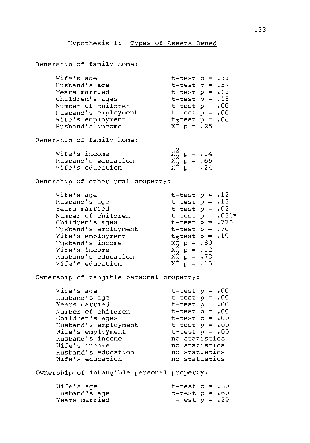
Hypothesis 1:
Types of Assets Owned
Ownership of family home:
Wife's age
Husband's age
Years married
Children's ages
Number of children
Husband's employment
Wife's employment
Husband's income
Ownership of family home:
Wife's income
Husband's education
Wife's education
Ownership of other real property:
Wife's age
Husband's age
Years married
Number of children
Children's ages
Husband's employment
Wife's employment
Husband's income
Wife's income
Husband's education
Wife's education
t-test p = .22
t-test p = .57
t-test p = .15
t-test p = .18
t-test p = .06
t-test p = .06
t2test p = .06
X p = .25
X
2
p = .14
X
2
2
p = .66
X p = .24
t-test p = .12
t-test p = .13
t-test p = .62
t-test p = .036*
t-test p = .776
t-test p = .70
t-test p = .19
X
2
p = .80
X
2
p = .12
X
2
p = .73
X p = .15
Ownership of tangible personal property:
Wife's age
Husband's age
Years married
Number of children
Children's ages
Husband's employment
Wife's employment
Husband's income
Wife's income
Husband's education
Wife's education
t-test p = .00
t-test p = .00
t-test p = .00
t-test p = .00
t-test p = .00
t-test p = .00
t-test p = .00
no statistics
no statistics
no statistics
no statistics
Ownership of intangible personal property:
Wife's age
Husband's age
Years married
t-test p = .80
t-test p = .60
t-test p = .29
133

134
Number of children
Children's ages
Husband's employment
Wife's employment
Wife's income
Husband's income
Husband's education
Wife's education
t-test
p =
.42
t-test
p =
.35
t-test p = .48
t
2
test
p = .01*
X
2
p = .24
X
2
p =
.09
X
2
p =
X
p =
.35
.00*
Hypothesis 2:
Net Dollar Value of Assets
Pearson correlation coefficients:
Wife's age
Husband's age
Years married
Wife's employment
Pearson correlation coefficients:
Husband's employment
Number of children
Children's ages
Children with wife
Net dollar value of assets:
Children with husband
Amount child support
Amount spousal support
Duration spousal support
Wife's income
Husband's income
Wife's education
Husband's education
p
p
p
p
= .007*
= .015*
= .005*
= .733
p = .122
p = .009*
p = .125
p
= .558
P
= .264
p = .001*
p = .064
p = .277
P
prob. = .53
F prob. = .80
F prob. = .74
F prob. = .95
Hypothesis 3:
Method of Valuation
Family home
Other real property
Cars
Other vehicles
Furniture
Bank accounts
Stocks/bonds/investments
Business/professional
practice
Insurance
Pension
2
X2
X
2
X
2
X2
X
2
2
X
2
X
X
2
X
2
X
2
p
p
p
p
p
p
p
p
p
=
=
=
=
=
=
=
=
=
=
.41
.63
.94
.13
1.0
.90
.56
.73
.41
.61

135
Any other asset
X
2
p = 1.0
Hypothesis 4: Asset Allocation
Who kept family home:
Wife's age
Husband's age
Years married
Wife's employment
Husband's employment
Children with wife
Children with husband
Amount child support
Amount spousal support
Duration spousal support
Assets minus debts
Wife's income
Husband's income
Wanted divorce-beginning
Wanted divorce-end
Who kept family home:
Wife's education
Husband's education
Who made decisions
Who kept other real property:
F prob. = .224
F prob. = .599
F prob. = .446
F prob. = .264
F prob. = .366
F prob. = .021*
F prob. = .011*
F prob. = .546
F prob. = .600
F prob. = .576
F
2
prob. = .637
X
2
p = .93
X p = .96
X
2
p = .15
X
2
p = .34
X
2
2
p = .84
X
2
p = .62
X p = .46
Wife's age E prob. = .049*
Husband's age
F prob. = .090
Years married F prob. = .048*
Wife's employment
F prob. = .995
Husband's employment F prob. = .054*
Children with wife F prob. = .944
Children with husband F prob. = .793
Amount child support F prob. = .949
Amount spousal support
F prob. = .587
Duration spousal support F prob. = .074
Assets minus debts F prob. = .263
Wife's income
X
2
p = .37
Husband's income
X
2
p = .49
Wanted divorce-beginning X
2
X2
p = .78
Wanted divorce-end X
2
p = .70
Wife's education
X
2
p = .61
Husband's education
X
2
p = .20
Who made decisions X p = .64

136
Who kept tangible personal property:
Wife's age
F prob.
Husband's age
F prob.
Years married
F prob.
Wife's employment
F prob.
Husband's employment
F prob.
Children with wife F prob.
Children with husband
F prob.
Amount child support
F prob.
Amount spousal support
F prob.
Duration spousal support
F prob.
Assets minus debts
F
2
prob.
Wife's income X
2
p =
Husband's income
X
2
p =
Wanted divorce-beginning
X
2
p =
Wanted divorce-end
X
2
p =
Wife's education
X
2
p =
Husband's education
X
2
p =
Who made decisions
X p =
= .679
= .510
= .761
= .162
= .988
= .008*
= .275
= .786
= .107
= .207
= .458
.02*
.11
.69
.025*
.87
.54
.93
Who kept intangible personal property:
Wife's age
F prob.
Husband's age
F prob.
Years married
F prob.
Wife's employment
F prob.
Husband's employment
F prob.
Children with wife
F prob.
Children with husband F prob.
Amount child support F prob.
Who kept intangible personal property:
Amount spousal support
F prob.
Duration spousal support F prob.
Assets minus debts F
2
prob.
Wife's income
X2
p =
Husband's income X
2
p =
Wanted divorce-beginning X
2
p =
Wanted divorce-end
X
2
2
p =
Wife's education X
2
p =
Husband's education
X
2
p =
Who made decisions
X p =
=
=
=
=
=
=
=
=
=
=
=
.43
.68
.65
.19
.70
.24
.46
.239
.868
.399
.439
.597
.839
.592
.893
.299
.403
.418
Hypothesis 5: Percentage of Assets to Wife
Pearson correlation coefficients
Wife's age p = .90
Husband's age p = .49

137
Years married
Wife's employment
Husband's employment
Children with wife
Children with husband
Amount child support
Amount spousal support
p
p
p
p
p
p
p
= .42
= .12
= .49
= .27
= .56
= .61
= .61
Duration spousal support p = .22
Assets minus debts p = .85
Wife's income F prob. = .841
Husband's income F prob. = .398
Wanted divorce-beginning F prob. = .554
Wanted divorce-end F prob. = .320
Wife's education F prob. = .954
Husband's education
F
prob. = .633
Who made decisions
F prob.
= .251
Family home owned F prob. = .029*
Tangible personal property
owned
no
statistics
Intangible personal
property owned
no statistics
Hypothesis 6: Post-Divorce Economic Well-Being
Stepwise Multiple Regression
Respondent presently
employed p = .036*
Respondent's age p = .101
Years married
p = .013*
Who made decisions p = .088
Respondent's net assets p = .196
Amount child support
p
=
.133
Respondent's education p = .239
Amount spousal support
p
=
.377
Respondent's sex
p
=
.236

138
V. IMPLICATIONS AND RECOMMENDATIONS
The purpose of this study was to provide data on
the economic aspects of divorce in Oregon after ten or
more years of marriage, with particular emphasis on the
valuation and allocation of assets.
The findings from
this exploratory study suggest the following conclusions:
Most couples divorcing after ten or more years
owned one major asset, the family home.
The parent
having custody of the minor children was most likely to
continue living in the family home.
Because mothers
were more likely to have the minor children living with
them, a higher percentage of residence awards were to
wives. However, the spouse remaining in the family home
was usually required to make installment payments to the
other spouse for his or her share of the equity. Given
the low incomes of most of these divorced women, their
ability to pay the other spouse seems doubtful, and an
eventual sale of the family home inevitable.
Respon-
dents owning homes in joint ownership with former
spouses reported problems in both sales and maintenance.
The resident owner reported having responsibility for
insurance, taxes, and upkeep and reported that the non-
resident owner could control the selling price and/or
make the selling process difficult.
Fewer children in the family increased the likeli-
hood of the family owning real estate other than a fam-

139
ily home.
It may be that families with fewer children
have more money available for investment in real estate,
or families with fewer children have more interest in
the tax advantages associated with owning real estate.
Tangible personal property, although owned by a
majority of couples, was usually assets with low mone-
tary values such as furniture and cars.
The dollar
value of the tangible personal property received by hus-
bands was greater in families with fewer children.
This
may reflect that when there are more children in the
family, tangible personal property was more likely to
be household furnishings and appliances and less likely
to be second cars or other vehicles.
As the educational level and number of years of
paid employment of wives increased, the ownership of
intangible personal property increased.
This may re-
flect that the wife's income provides the margin enabl-
ing the family to invest.
Or it may reflect that women
with more education and more years in the paid labor
force have pensions--one item included in the category
"intangible personal property." Ownership of pensions,
and their values, varied greatly by gender.
Husbands
were more likely than wives to have acquired pensions
during the marriage.
When both husband and wife had pensions, the hus-
band's was of higher value.
Even though most of the di-
vorcing couples had some savings in bank accounts, their

140
account values were very low.
One of the major decisions couples must make at di-
vorce is how to value and divide existing assets.
Oregon is an all-asset equitable distribution state re-
quiring that real and personal property be divided as
may be "just and proper in all the circumstances."
About half of these divorcing couples reported valuing
and allocating their common possessions in "kitchen-
table" negotiations.
When couples were homeowners, assets were divided
almost equally between husbands and wives.
When a fam-
ily home was not owned, wives retained a greater percent-
age of the couple's net assets.
However, since the fam-
ily home was likely to be the most valuable asset, when
there was no homeownership, total assets had low values.
Therefore, the cases in which wives received a large
percentage of the assets were likely to be the cases
with the lowest asset values.
When the net dollar value of assets (assets minus
debts) retained by wives and by husbands were examined,
the median value of wife's net assets was $28,850, and
husband's, $24,908, indicating that assets were being
divided fairly evenly.
In the majority of cases, values of property were
determined by the husband and wife regardless of whe-
ther the couple themselves divided the assets or the
property settlement was negotiated by attorneys.
The

141
higher value an asset had, the more likely it was to
have been objectively valued (some data used to arrive
at the value). Family homes, other real property, bank
accounts, stocks and bonds and "any other assets" were
valued objectively about half of the time. Business/pro-
fessional practices and insurance policies were valued
objectively somewhat less than half of the time.
Cars
and other vehicles were valued objectively less than a
third of the time.
Furniture was rarely valued objec-
tively.
About two-thirds of the couples owned pensions
or retirement accounts. These were frequently of great
value and valued objectively by less than one-third of
the couples. Often, in the case of pensions, the re-
spondent would say, "I had mine and she/he had hers/his,"
without looking at the differences in length of employ-
ment, earnings, and future benefits.
In most instances,
couples needed assistance in determining asset values
and in understanding the differences between present and
future values.
This was true not only for pensions but
also for family homes with equity judgements.
One of the most interesting and unexpected findings
from the interviews involved participant answers to the
question, "When you reach retirement age, how likely are
you to have your own Social Security benefits?" Many
respondents believed the question to be related to the

142
continuation of the Social Security system and answered,
"Not very likely."
Sixty-three percent of the husbands
had pensions or other retirement plans in addition to
Social Security benefits, but only 29 percent of the
wives had alternate retirement accounts.
Social Secu-
rity benefits have become the primary or sole source of
income for millions of retirees.
But Social Security
alone is not intended to maintain preretirement living
standards. Private pensions and personal savings are
supposed to contribute substantially to retirement in-
come. Even though a retired individual's needs are
less, they will still need between 55 and 78 percent of
gross preretirement income.
In addition, women have
special needs associated with longevity.
The need for
preretirement educational programs to help women and
men plan for the future is evident.
Although most couples shared liabilities, husbands
were assuming a larger percentage of the family debt
than were wives ($6,296 and $1,870, respectively).
However, husbands also had higher incomes even after the
subtraction of spousal support and/or child support ob-
ligations, so husbands had more ability to repay.
Wom-
en's incomes after divorce, even after the addition of
spousal support and/or child support payments, were con-
sistently lower than men's incomes.
While the amounts of the property awards is a concern
that cannot be ignored, an equally important concern is

143
the lack of income-earning ability of the wives.
In
many instances there was not enough family property to
be divided or enough spousal support which could be
awarded to compensate for the low income status of the
divorced woman.
A greater awareness of financial management during
marriage could help alleviate serious problems at dis-
solution.
As one respondent said, "One of the biggest
problems in our marriage was economics."
Many respon-
dents who had been in two-earner marriages, particularly
when they had been using credit extensively, mentioned
how hard it was to manage on only one income.
In addi-
tion, many respondents were uncertain about such basic
details of family finances as annual net income, family
debts, and monthly cash flow.
It was the norm for one
spouse to handle all the family finances.
Then, when
divorce occurred, the other spouse expressed a strong
need for financial counseling to assist them in
straightening out complex debt problems and to learn how
to manage their money.
Efforts should be made to expand
financial management education in high schools, colleges,
and adult education programs.
Few wives received spousal support, and most sup-
port orders were for a short, fixed duration.
The medi-
an amount of spousal support was $400 a month for three
years.
These minimal support awards created severe
hardships for many of the women, especially those who

144
had been full-time homemakers during most of the mar-
riage.
Without occupational or professional training
and labor market experience, they were compelled to take
entry level, low-paying positions to meet short-term
necessities.
They also faced divorce with the loss of
benefits, such as health care coverage and pensions.
Women today, married or not, will work at paid employ-
ment throughout most of their adult years.
One clear
implication is the need for career/life planning for
young women to help them maximize their earning capac-
ities.
In the majority of cases, dependent children were
in the custodial care of the mother.
There was a small,
but meaningful, trend toward fathers having custody of
minor children and toward joint or split custody.
Co-
parenting took many forms; sometimes joint custody meant
both physical and legal custody, in some cases one par-
ent was designated as the primary physical custodian,
and some couples separated the children and both parents
had children in their custody.
Child custody was a spe-
cial source of frustration for many fathers; who indicat-
ed that the most difficult aspect of divorce was separa-
tion from their children.
Child support was usually awarded if there were
children under the age of 18, and almost always it was
paid by fathers.
A small percentage of mothers without
custody were obligated to pay child support.
The median

145
amount of child support was $188.50 per month.
At the
time these divorces were finalized, the annual cost of
raising a 10 or 11 year old child (the average age of
minor children in this study) in the West at a moderate
cost level was $5,302, or $441.83 per month (Family
Economics Review, 1985).
Half of this monthly estimate
is $220.92. Therefore the median amount of child sup-
port was less than half the cost of raising the child.
The amount of child support is rarely modified upward.
Since the cost of raising children increases with infla-
tion and the child's age, support orders are eroded.
Over time custodial parents assume a disproportionate
share of the costs of raising their children. When
child support orders are evaluated in terms of each par-
ent's ability to pay, mothers typically assume the lar-
ger share of the costs of raising their children.
In
most calculations of the cost of raising children, the
major child care expenses borne by the custodial parent
are rarely taken into account.
Often for the mother
employed full-time, the cost of child care alone equals
or exceeds the child support order.
To quote one work-
ing mother, "The cost of child care is a killer."
Yet
requests for child and/or spousal support awards were
seldom accompanied by clear or convincing proof of fam-
ily expenses.
There was an uneven relationship between husband's
and wife's post-divorce income, even after all income

146
transfers were subtracted or added. Fifty-five percent
of the wives had "adjusted" annual incomes below $20,000
compared to 24 percent of the husbands.
Seventy-five
percent of the husbands had incomes above $20,000; 49
percent of them had post-divorce incomes of $30,000 or
more. While both parties were affected financially in
the short term, it is clear that the relative impact was
greater for the wife and children.
Because 'we more readily understand tangible assets
than potential future income, it is easy to conclude
that a 50-50 division of a couple's home, furniture,
cars, and bank accounts fulfills equity between the
spouses.
However, it is clear from the adjusted post-
divorce income figures that this "equality" structures
different economic futures for wives and husbands after
divorce.
Most policy makers do not take into consider-
ation all of the economic consequences of divorce and
therefore have not recognized needed changes.
The four
specific policy changes that follow would help remove
some of the inequities of the current laws and proce-
dures.
1) Legislation is needed requiring judges to consider
nonmonetary contributions to a marriage in the same man-
ner as are the monetary contributions.
The long-married
homemaker, has assumed most of the "family" duties
allowing the other spouse to develop earning potential.
Rules are needed that redistribute post-divorce income

147
with the goal of providing the homemaker-spouse an ade-
quate level of living.
This would protect those spouses
who have devoted most of their lives to home and child-
ren, and in so doing did not develop their own earning
capacities.
2) Financial assistance is needed by custodial parents.
Child support awards should provide for adequate housing
and the other financial needs of the child. Support
awards should include ways to adjust the support order
as prices increase, as parents' incomes change, and the
financial needs associated with raising children change.
The in-kind contributions of homemaking and child care
should be considered support by the custodial parent.
Continued and enhanced efforts are needed to enforce
the payment of child support.
3) Greater attention needs to be paid to the employ-
ment possibilities and compensation of divorced women.
In the awarding of "rehabilitative alimony" there is
rarely a realistic evaluation of the difficulties women
have finding reasonable, fairly compensated employment,
especially after an absence from the labor market. A
greater expectation of self-sufficiency is expected from
women after divorce, and the need for them to provide for
themselves and their dependent children at a time when
equality is lacking in employment opportunity, job prep-
aration, and salaries.
What is needed are spousal sup-
port awards that allow for career counseling and retrain-

148
ing following divorce.
4) Young women should be encouraged to
explore a wide range of career options to avoid the trap
of concentration in low paying, dead-end jobs.
They
should be well informed about the need for developing
financial independence, not only in order to avoid the
financial pitfalls often encountered in divorce, but to
help move closer to the concept of marriage as a true
partnership.
Recommendations for Further Study
Much, if not all, that we know about the economic
consequences of divorce has been gathered from cross-
sectional studies on urban populations. More informa-
tion is needed on rural farm families.
Case law (Haque-
wood and Haquewood, 1981) suggests that farm families
may have special considerations because the major asset
is an ongoing business from which both parties receive
financial security.
Little can be concluded with certainty about the
long-term effects of divorce. With the exception of
Wallerstein and Kelly's (1980) research on the effects
of divorce on children, and the Panel Survey of Income
Dynamics ten-year research project on five thousand
American families, good longitudinal studies are almost
nonexistent. Longitudinal studies on divorce would con-
tribute necessary information.

149
It has been suggested that it costs more to raise
a child in a one-parent family than an intact, two-
parent family, partly because of the cost of child care
and partly because of losses of economics of scale in
smaller living units.
Expenditure surveys of single-
parent families are needed.
Any replication of this study would profit from
recategorization of asset categories.
"Tangible per-
sonal property" and "intangible personal property" were
too inclusive to yield the most useful data.
A better
classification might be "consumer use assets" and "in-
vestment assets."
In terms of post-divorce economic
well-being, there is a difference between a consumer use
asset such as a $10,000 automobile which will depreciate
and an investment asset such as $10,000 worth of stock
which may increase in value as well as produce income.
At the present time, the courts use, in large mea-
sure, valuation and allocation of assets to insure that
each of the parties separate on an equitable a basis as
is possible.
Additional measures of future economic
well-being are the ability to earn income, access to
credit, and/or recent education/training.
The impor-
tance of these factors needs to be investigated.
Federal laws that went into effect in October 1984
and October 1985, require all states to enforce child
support payments both for parents with children on wel-
fare and for families not on public assistance.
Data

150
are needed on noncompliance before and after these laws
became effective.
Most divorce studies utilize samples drawn from
local populations. While such information is useful,
the differences in state laws make generalizations to
the population as a whole less useful. Replication of
existing studies in states with other marital property
laws is needed.
In future studies related to property settlements,
inclusion of an "equity measure" from social exchange
theory could be developed.
A body of literature exists
which tells us when individuals perceive themselves in
a relationship with, and compare their outcomes with,
others. Anecdotal data confirms that this relationship
exists after divorce.
In the future, it could be prof-
itable to attempt to relate this to equity theory.
General systems theory could be useful in future
studies on divorce. A family system changes, but does
not end, when divorce occurs. Therefore, investigation
of the changes in this system as well as on new and over-
lapping changes which are created by separated families
should prove fruitful.

151
TABLE OF CASES
Baker v. Baker, 16 App. Div. 2d 409, 228 N.Y.S.2d 470
(1962).
Commonwealth v. George, 358 Pa. 118, 56 A.2d 228 (1948).
Doyle v. Doyle, 5 Misc. 2d 4, 158 N.Y.S.2d 909 (1957).
Ewell v. State, 207 Md. 288, 14 A.2d 6.6 (1955).
Garlock v. Garlock, 279 N.Y. 337, 18 N.E. 2d 251 (1939).
Glatt v. Glatt, 41 Or. App. 615, 598 P.2d 1237 (1979).
Grove v. Grove, 280 Or. 341, 571 P.2d 477 (1977).
Haguewood v. Haquewood, 292 Or 197, 638 P2d 1135 (1981).
In re Gaub, 25 Or App 107, 548 P.2d 178 (1976).
Johnson v. Johnson, 245 Or. 10, 419 P.2d 28 (1966).
Kitson v. Kitson, 17 Or. App. 648, 523 P.2d 575 (1974).
McCraw v. McCraw, 231 Or. 638, 373 P.2d 667 (1962).
Morgan v. Morgan, 13 Or. App. 14, 507 P.2d 409 (1973).
Orr v. Orr, 440 U.S. 268 (1979).
Poffenberger v. Poffenberger, 72 Md. 321, 19 A. 1043
(1980).
Ray v. Ray, 11 Or. App. 246, 502 P.2d 397 (1972).
Rothman v. Rothman, 65 N.J. 228, 320 A.2d 501 (1974).
Rucci v. Rucci, 23 Conn. Supp. 221, 181 A.2d 125 (1962).
Siebert v. Siebert, 184 Or. 496, 199 P.2d 659 (1948).
Smith v. Smith, 290 Or. 675, 626 P.2d 342 (1981).
Tinqen v. Tingen, 251 Or. 458, 446 P.2d 185 (1968).
Wirth v. Wirth, 38 App. Div. 2d 611, 326 N.Y.S.2d 308
(1971).

152
REFERENCES
Aarnas, Laila E. "Family Law--Determination of Spousal
Support: Grove and Grove."
57 Oregon Law Review
566 (1978).
Adams, Chester H. "The Judiciary and Child Support."
Juvenile and Family Court Journal 1 (February
1983):5.
Albrecht, Stan L.
"Reactions and Adjustments to Divorce:
Differences in the Experiences of Males and
Females." Family Relations 29 (January 1980):59.
Allen, Edward; "Smith vs. Smith: The Debate Continues."
10 Oregon Trial Lawyer 7 (1982).
Bahr, Stephen J. "Marital Dissolution Laws: Impact of
Recent Changes on Women." Journal of Family Issues
4 (September 1983):455.
Bane, Mary Jo. "Marital Disruption and the Lives of
Children." Journal of Social Issues 32 (January
1976):103.
Bartke, Richard, and Zurvalec, Lori A. "The Low, Middle
and High Road to Marital Property Law Reform in
Common Law Jurisdictions." 7 Community Property
Journal 200 (1980).
Bernard, Jessie. "No News, But New Ideas." In Divorce
and After, pp 3-29. Edited by Paul Bohannan, New
York: Doubleday and Co., 1971.
Black, Henry Campbell. Black's Law Dictionary. 5th ed.
St. Paul: West Publishing Co., 1983.
Brake, Stephen J.
"Equitable Distribution vs. Fixed
Rules: Marital Property Reform and the Uniform
Marital Property Act."
23 Boston College Law
Review 761 (1982).
Brandwein, Ruth A.; Brown, Carol A.; and Fox, Elizabeth
M. "Women and Children Last: The Social Situation
of Divorced Mothers and Their Families." Journal
of Marriage and the Family 36 (August 1974):498.
Cantwell, William P.
"Man + Woman + Property = ? --
Pondering the Marital Equation." 6 Probate Lawyer
1 (1980).

153
Caudle, Shelia.
"Women Left Behind in Our War on
Poverty."
Statesman Journal, 8 August 1982,
sec. A, p. Al.
Carter, Hugh, and Glick, Paul C.
Marriage and Divorce:
A Social-Economic Study.
Cambridge: Harvard
University Press, 1970.
Cassety, Judith.
Child Support and Public Policy:
Securing Support from Absent Fathers.
Lexington,
Mass.: Lexington Books, 1978.
Cheadle, Elizabeth A.
"The Development of Sharing
Principles in Common Law Marital Property States."
28 UCLA Law Review 1269 (1981).
Clark, Homer..
The Law of Domestic Relations.
St. Paul:
West Publishing Co., 1968.
Collins, Glenn.
"Fathers Who Don't Support Their
Children Spark Debate Nationwide."
The Oregonian,
8 November 1983, sec. C, p. Cl.
Connell, Mary J.
"Property Division and Alimony Awards:
A Survey of Statutory Limitations on Judicial
Discretion."
50 Fordham Law Review 415 (1981).
Corbett, Richard B.; Fethke, Carol C.; and Hauserman,
Nancy R.
"Achieving Economic Justice for Home-
makers."
Journal of Home Economics 72 (Summer
1980):17.
Crozier, Blanche.
"Marital Support" 15 Boston Univer-
sity Law Review 28 (1935)
Cutright, Phillips.
"Components of Change in the Number
of Female Family Heads Aged 15-44: United States,
1940-1970."
Journal of Marriage and the Family 36
(November 1974):714.
Derdeyn, Andre P.
"Child Custody: A Reflection of
Cultural Change."
Journal of Clinical Child
Psychology 7 (Fall 1978):169.
DiLeo, Louis M. J., and Model, Erick L.
"A Survey of
the Law of Property Disposition Upon Divorce in
the TriState Area."
56 St. John's Law Review 219
(1982).
Divorces and Annulments by Duration of Marriage in Years
1975-1982.
Portland, Oregon:
Oregon State Health
Division, Vital Statistics Section.

154
Dixon, Ruth B. and Weitzman, Lenore J.
"When Husbands
File for Divorce."
Journal of Marriage and the
Family 44 (February 1982):103.
Dullea, Georgia.
"Divorce."
New York Times News Ser-
vice 4 August 1985.
Eckhardt, Kenneth W.
"Deviance, Visibility, and Legal
Action: The Duty to Support."
Social Problems 15
(Spring 1968):470.
Eden, Philip.
"How Inflation Flaunts the Court's
Order."
1 Family Advocate 2 (1979).
Eisler, Riane T.
Dissolution: No-Fault Divorce, Mar-
riage and the Future of Women.
New York:
McGraw
Hill, 19-77.
Emberson, Heather.
"Average Annual Budgets for a Family
of Four at Four Income Levels."
Paper presented at
Oregon State University, Corvallis, Oregon, 1981.
Espenshade, Thomas J.
"The Economic Consequences of
Divorce."
Journal of Marriage and the Family 41
(August 1979):615.
Family Law Reporter.
Desk Guide to the Uniform Marriage
and Divorce Act.
Rockville, Maryland:
BNA Books,
1982.
Fetterly, Patricia.
"Oregon Marital Property Laws: Can
Both Separation and Equality Be Achieved?"
57
Oregon Law Review 152 (1977).
Folberg, H. Jay, and Graham, Marva.
"Joint Custody of
Children Following Divorce."
12 University of
California-Davis Law Review 523 (1979).
Foster, Henry H., Jr.
"Alimony Awards."
In Economics
of Divorce: A Collection of Papers, pp 1-19.
Chicago:
Section of Family Law, American Bar
Association, 1978.
Foster, Henry H., Jr., and Doris J. Freed.
"Life With
Father: 1978."
11 Family Law Quarterly 321 (1977).
Foster, Henry H., Jr., and Doris J. Freed.
"Marital
Property Reform in New York: Partnership of Co-
Equals?"
S Family Law Quarterly 169 (1974).
Foster, Henry H., Jr.; Freed, Doris J.; and Midonick,
Millard L.
"Child Support: The Quick and the
Dead."
26 Syracuse Law Review 1157 (1975).

Freed, Doris J., and Foster,
in the Fifty States: An
Quarterly 289 (1983).
Freed, Doris J., and Foster,
in the Fifty States: An
Quarterly 365 (1984).
Freed, Doris J., and Walker, Timothy B.
"Family Law in
the Fifty States: An Overview."
18 Family Law
Quarterly 369 (1985).
Henry H., Jr.
Overview." 16
Henry H., Jr.
Overview."
17
155
"Family Law
Family Law
"Family Law
Family Law
Friedman, Lawrence M., and Percival, Robert V.
"Who
Sues for Divorce?
From Fault Through Fiction to
Freedom."
5 Journal of Legal Studies 61 (1976).
Gates, Margaret.
"Homemakers Into Widows and Divorcees:
Can the Law Provide Economic Protection?"
In Women
Into Wives: Legal and Economic Impact of Marriage.
pp 215-232.
Edited by Jane Roberts Chapman and
Margaret Gates.
Beverly Hills:
Sage Publications,
1977.
Giele, Janet Z. "Changing Sex Roles and Changing Fami-
lies."
In Current Issues in Marriage and the Fam-
ily, pp 125-140.
Edited by J. Gipson Wells. New
York:
MacMillan Publishing Co., Inc., 1983.
Gildea, Larry O.
Report to Domestic Relations Seminar,
Oregon Trial Lawyer's Association, 18 April 1981,
Eugene, Oregon.
Glendon, Mary A.
"Modern Marriage Law and Its Under-
lying Assumptions: The New Marriage and the New
Property."
12 Family Law Quarterly 441 (1980).
Golden, Lawrence J.
Equitable Distribution of Property.
Colorado Springs, Colorado:
Shepard's/McGraw-Hill
(1983).
Goldstein, Joseph; Freud, Anna; and Solnit, Albert J.
Beyond the Best Interests of the Child.
New York:
The Free Press (1973).
Goode, W. J. After Divorce.
New York: Free Press,
1956.
Governor's Commission on Child Support Enforcement, by
Leonard Systma, Chairman.
Child Support Program,
Adult and Family Services Division, Salem, Oregon
(October 1985).

156
Graham, Kathy T.
"Domestic Relations."
Willamette
University, Salem, Oregon, 1983.
(Mimeographed)
Gravatt, Arthur E., and Hunt, Shirley P.
Oregon Family
Profile.
Corvallis:
Family Study and Research
Center, Oregon State University, 1979.
Greene, Rita.
"Property Settlements in Divorce Pro-
ceedings: Patterson v. Patterson."
84 West
Virginia Law Review 457 (1982).
Greene, Scott.
"Comparison of the Property Aspects of
the Community Property and Common Law Marital Prop-
erty Systems and Their Relative Compatibility with
the Current View of the Marriage Relationship and
the Rights of Women."
13 Creighton Law Review 71
(1979).
.
Gunter, B. B.
"Notes on Divorce Filing as Role Be-
havior."
Journal of Marriage and the Family 39
(February, 1977):95.
Gunter, B. G., and Johnson, D. P.
"Divorce Filing as
Role Behavior: Effect of No-Fault Divorce Filing
Patterns."
Journal of Marriage and the Family 40
(August, 1978):571.
Halem, Lynne C.
Divorce Reform: Changing Legal and
Social Perspectives.
New York:
The Free Press,
1980.
Hayghe, Howard.
"Marital and Family Patterns of
Workers: An Update."
Monthly Labor Review 105
(May 1982):53.
Hoffman, Saul.
"Marital Instability and the Economic
Status of Women."
Demography 14 (February 1977):
67.
Hoffman, Saul, and Holmes, John.
"Husbands, Wives, and
Divorce."
In Five Thousand American Families- -
Patterns of Economic Progress (Vol. 4), pp 163-
187. Edited by Greg J. Duncan and James N. Morgan.
Ann Arbor:
Institute for Social Research, Univer-
sity of Michigan, 1976.
Hogoboom, William P.
"The California Family Law Act of
1970: 18 Months' Experience."
27 Journal of
Missouri Bar 584 (1971).
Hortsch, Dan.
"Child Support, Custody Hashed Over at
State Airing."
The Oregonian, 6 March 1985, sec.
B, p B10.

157
Johnson, Beverly L. "Women Who Head Families, 1970-
1977: Their Numbers Rose, Income Lagged." Monthly
Labor Review 101 (February 1978):32.
Johnson, Beverly L. "Single Parent Families."
Family
Economics Review (Summer/Fall 1980):22.
Johnson, Beverly L., and Waldman, Elizabeth. "Marital
and Family Patterns of the Labor Force." Monthly
Labor Review 104 (October 1981):36.
Johnston, John D., Jr. "Sex and Property: The Common
Law Tradition, The Law School Curriculum, and
Developments Toward Equality."
47 New York Univer-
sity Law Review 1033 (1972).
Jones, Carol Adaire; Gordon, Nancy M.; and Sawhill,
Isabel V.
Child Support Payments in the U. S.:
Urban Institute Working Paper 992-03.
Washington
D. C.:
The Urban Institute, 1976.
Joseph, Marjory L., and Joseph, William D.
Research
Fundamentals in Home Economics.
Redondo Beach,
California:
Plycon Press, 1979.
Kanowitz, Leo.
Women and the Law: The Unfinished Revo-
lution. Albuquerque: University of New Mexico
Press, 1969.
Karowe, Marjorie E. "Marital Property: A New Look at
Old Inequities."
39 Albany Law Review 52 (1974).
Kay, Herma Hill.
"A Family Court: The California Pro-
posal." In Divorce and After, pp 243-281.
Edited
by Paul Bohannan.
New York: Doubleday and Co.,
1971.
Kay, Herma Hill.
"Making Marriage and Divorce Safe for
Women."
60 California Law Review 1683 (1972).
Kitagawa, Evelyn M.
"New Life-Styles: Marriage Pat-
terns, Living Arrangements, and Fertility Outside
of Marriage."
Annals of the American Academy of
Political and Social Science. 453 (January 1981):
1.
Kitson, Gay C., and Raschke, Helen J. "Divorce Research:
What We Know; What We Need to Know."
Journal of
Divorce 4 (Spring 1981):1.
Krause, Harry D.
Family Law. St. Paul: West Publish-
ing Co., 1981.

Krauskopf, Joan.
Needed."
In
nomic Impact
Jane Roberts
Hills:
Sage
158
"Partnership Marriage: Legal Reforms
Women Into Wives: The Legal and Eco-
of Marriage, pp 93-121.
Edited by
Chapman and Margaret Gates.
Beverly
Publications, 1977.
Krauskopf, Joan M., and Thomas, Rhonda C. "Partnership
Marriage: The Solution to an Ineffective and In-
equitable Law of Support."
35 Ohio State Law
Journal 558 (1974).
Kressel, Kenneth; Lopez-Morillas, Martin; Weinglass,
Janet; and Deutsch, Morton.
"Professional Inter-
vention in Divorce: A Summary of the Views of
Lawyers, Psychotherapists, and Clergy."
Journal
of Divorce 2 (Winter 1978):119.
Kriesberg, Louis.
Mothers in Poverty: A Study of
Fatherless Families. Chicago:
Aldine Publishing
Co., 1970.
Kulzer, Barbara A.
"Law and the Housewife: Property,
Divorce, and Death."
28 University of Florida Law
Review 1 (1975).
Larson, Bianca G.
"Equity and Economics: A Case for
Spousal Support."
8 Women's Law Forum 443 (1979).
Leo, Roger J.
"Oregon's No-Fault Marriage Dissolution
Act."
51 Oregon Law Review 715 (1972).
Levitan, =1,12:;:andaBeITI314n:i2I2mTly "Working
Monthly
Labor Review 104 (September 1981):26.
Interview with John J. Luck,
sion, Oregon Department
Oregon, 3 April 1985.
Mandelker, Daniel R.
"Family
American Poor Laws: I."
497 (1956).
Support Enforcement Divi-
of Justice, Portland,
Responsibility Under the
54 Michigan Law Review
Marsden, Dennis.
Mothers Alone: Poverty and the Father-
less Family.
London:
The Penguin Press, 1969.
McCormack, Patricia.
"Poverty in Families Headed by
Women."
United Press International 12 March 1985.
McEaddy, Beverly J.
"Women Who Head Families: A Socio-
economic Analysis."
Monthly Labor Review 99 (June
1976):3.

159
McGraw, Robert E.; Sterin, Gloria J.; and Davis, Joseph
M.
"A Case Study in Divorce Law Reform and Its
Aftermath."
20 Journal of Family Law 443 (1982).
Mellor, Earl F., and Stamas, George D.
"Usual Weekly
Earnings: Another Look at Intergroup Differences
and Basic Trends."
Monthly Labor Review 105 (April
1982):15.
Milkovich, George T.
"The Male-Female Pay Gap: Need
for Reevaluation." Monthly Labor Review 104 (April
1981):42.
Mnookin, Robert H. "Child Custody Adjudication:
Judi-
cial Functions in the Face of Indeterminancy." 39
Law and Contemporary Problems.
(Summer 1975):226.
Morris, Earl W. and Winter, Mary. Housing, Family and
Society. New York: John Wiley and Sons, 1978.
Mott, Frank L., and Moore, Sylvia F. The Socioeconomic
Status of Households Headed by Women. R & D Mono-
graph 72, U. S. Department of Labor, Employment
and Training Administration, Government Printing
Office, Washington, D. C., 1979.
Murphy, Michael C. "The Implied Partnership: Equitable
Alternative to Contemporary Methods of Postmarital
Property Distribution." 26 University of Florida
Law Review 226 (1974).
Neter, John; Wasserman, William; and Kutner, Michael H.
Applied Linear Regression Models. Homewood,
Illinois: Richard D. Irwin, 1983.
Norton, Arthur J., and Glick, Paul C. "Marital Insta-
bility: Past, Present, and Future." Journal of
Social Issues 32 (1976):5.
O'Donnell, Martha.
"Smith v. Smith: No Magic Formula
for Determining Child Support Payments of the Non-
custodial Parent." 18 Willamette Law Review 353
(1982).
Oregon Blue Book: 1983-84. Forest Grove, Oregon: Times
Litho (1983).
Oregon Revised Statutes 107.005 - 107.830 (1983 Replace-
ment Part).
Oregon Public Health Statistics Report for Calendar Year
1980. Portland, Oregon:
Oregon State Health Divi-
sion, Vital Statistics Section.
160
Patterson, Michelle.
"What's Yours is Mine and What's
Mine is Mine: The Classification of the Home Upon
Dissolution."
28 UCLA Law Review 1365 (1981).
Perlman, Richard.
The Economics of Poverty.
New York:
McGraw-Hill Book Co., 1976.
Podell, Ralph J.
"The Case for Revision of the Uniform
Marriage and Divorce Act."
7 Family Law Quarterly
169 (1973).
Prager, Susan Westerberg.
"Sharing Principles and the
Future of Marital Property Law."
25 UCLA Law
Review 1 (1977).
Price-Bonham, Sharon and Balswick, Jack O.
"The Non-
institutons: Divorce, Desertion, and Remarriage."
Journal of Marriage and the Family 42 (November
1980):959.
Rice, David G.
"Psychotherapeutic Treatment of Narcis-
sistic Injury in Marital Separation and Divorce,"
Journal of Divorce 1 (Winter 1977):119.
Rheinstein, Max.
Marriage Stability, Divorce and the
Law. Chicago:
University of Chicago Press, 1972.
Ross, Heather L., and Sawhill, Isabel V.
Time of Tran-
sition: The Growth of Families Headed by Women.
Washington, D. C.: The Urban Institute, 1975.
Sassower, Doris.
Testimony Before Joint Hearings of the
Matrimonial Law Committees of the New York County
Lawyers' Association and the'Association of the Bar
of the City of New York, 14 January 1972.
Schulman, Joanne and Pitt, Valerie. "Second Thoughts
on Joint Custody: Analysis of Legislation and its
Implications for Women and Children."
12 Golden
Gate University Law Review 539 (1982).
Seal, Karen.
"A Decade of No-Fault Divorce."
1 Family
Advocate 10 (1979).
"South Dakota No-Fault Divorce."
Americans for Legal
Reform, 6 Fall 1985, p 13.
Smith, Jeanne W., and Elizabeth S. Beninger.
"Women's
Nonmarket Labor: Dissolution of Marriage and Oppor-
tunity Cost."
Journal of Family Issues 3 (June
1982):251.

161
Smith, Michael J.
"Economic Conditions in Single-Parent
Families: A Longitudinal Perspective." Social Work
Research and Abstracts 16 (February 1980):20.
Stein, Robert L.
"The Economic Status of Families Head-
ed by Women." Monthly Labor Review 93 (December
1970):3.
Stevenson, Victoria.
"Oregon's No-Fault Divorce Law:
Effect on Custody, Property Division and Support."
55 Oregon Law Review 267 (1976).
Turnquist, Kristi. "Divorce Laws: A Question of
Balance." Willamette Week, 12-18 April 1983, p 4.
"Updated Estimates of Cost of Raising a Child." Family
Economics Review 2 (April 1985):32.
U. S. Bureau of the Census, Current Population Reports,
Series P-23, No. 112, Child Support and Alimony:
1981, U. S. Government Printing Office, Washington,
D. C., 1983.
U. S. Bureau of the Census,
Series P-23, No. 107,
Householders: 1970-79,
Office, Washington, D.
Current Population Reports,
Families Maintained by Female
U. S. Government Printing
C., 1980.
U. S. Bureau of the Census, Current Population Reports,
Series P-20, No. 380, Marital Status and Living
Arrangements: March 1982, U. S. Government Printing
Office, Washington, D. C., 1983.
U. S. Bureau of the Census, Current Population Reports,
Series P-60, No. 134, Money Income and Poverty
Status of Families and Persons in the United
States: 1981, U. S. Government Printing Office,
Washington, D. C., 1982.
U. S. Bureau of the Census, Statistical Abstract of the
United States: 1982-83, (104st Edition) U. S.
Government Printing Office, Washington, D. C., 1983.
U. S., Congress, House, Representative Martha Griffiths
speaking on Child Support Collection Among Welfare
Families, H. B. 11291, Congressional Record, 4
December 1974.
U. S. Department of
Bulletin 2080,
Databook, U. S.
ington, D. C.,
Labor, Bureau of Labor Statistics,
Perspectives on Working Women: A
Government Printing Office, Wash-
1981.

162
U. S. Department of Labor, Bureau of Labor Statistics,
Bulletin 1570-2, Three Budgets for an Urban Family
of Four: Autumn 1977, U. S. Government Printing
Office, Washington, D. C., 1968.
U. S. Department of Labor, Citizens Advisory Council on
the Status of Women, The Equal Rights Amendment and
Alimony and Child Support Laws.
U. S. Government
Printing Office, Washington, D. C., 1972.
U. S. Department of State, National Commission on the
Observance of International Women's Year, "...To
Form a More Perfect Union..." Justice for American
Women, U. S. Government Printing Office, Washington,
D. C., 1975.
Veith, Nancy A. "Rehabilitative Spousal Support: In
Need of a More Comprehensive Approach to Mitigating
Dissolution Trauma." 12 University of San Fran-
cisco Law Review 493 (1978).
Vernier, Chester G., and Hurlburt, John B. "The His-
torical Background of Alimony Law and Its Present
Statutory Structure."
6 Law and Contemporary
Problems 197 (1939).
Vickery, Clair. "Economics and the Single-Mother
Family."
Public Welfare. 36 (Winter 1978):18.
Wallerstein, Judith S., and Kelly, Joan B. Surviving
the Breakup: How Children and Parents Cope with
Divorce.
New York:
Basic Books, 1980.
Warren, C. A. B., and Rasmussen, P. K. "Sex and Gender
in Field Research."
Urban Life 6 (1977):349.
Wattenberg, Esther, and Reinhardt, Hazel. "Female-
Headed Families: Trends and Implications." Social
Work 24 (November 1979):460.
Weiss, Robert S. Marital Separation. New York: Basic
Books, 1975.
Weitzman, Lenore J. "No-Fault Divorce is 'Disaster'
for Wives, Children." The Salt Lake Tribune, 3
October 1985, sec. A, p Al.
Weitzman, Lenore J. "The Economics of Divorce: Social
and Economic Consequences of Property, Alimony and
Child Support Awards."
28 UCLA Law Review 1181
(1981).

163
Weitzman, Lenore J. The Marriage Contract: A Guide to
Living With Lovers and Spouses.
New York:
The
Free Press, 1981.
Weitzman, Lenore J., and Dixon, Ruth B. "Child Custody
Awards: Legal Standards and Empirical Patterns for
Child Custody, Support and Visitation After Di-
vorce." 12 University of California, Davis, Law
Review 473 (1979).
Weitzman, Lenore J., and Dixon, Ruth B. "The Alimony
Myth: Does No-Fault Make a Difference?" 14 Family
Law Quarterly 141 (1980).
Weitzman, Lenore J., and Dixon, Ruth B. "The Transfor-
mation of Legal Marriage Through No-Fault Divorce."
In Current Issues in Marriage and the Family, 3rd
ed., pp 217-232. Edited by J. Gipson Wells. New
York: Macmillan Publishing Co., 1983.
Winston, Marian, and Forsher, Trude. Nonsupport of
Legitimate Children by Affluent Fathers as a Cause
of Poverty and Welfare Dependence. Paper repro-
duced by the Rand Corporation, 1971.
Williams, Helenjane, Coordinator, Oregon Older Women's
Caucus, personal correspondence, 24 January 1984.
Wiseman, Reva S. "Crisis Theory and the Process of
Divorce."
Social Casework 56 (April 1975):212.
Wohler, Milly. "Women 'Astonished' at Many Victories
in '77 Legislature." The Oregonian, 29 P.2d 659
(1948).
Yee, Lucy M. "What Really Happens in Child Support
Cases: An Empirical Study of Establishment and En-
forcement of Child Support Orders in the Denver
District Court." 57 Denver Law Journal 21 (1979).
Younger, Judith T. "Community Property, Women and the
Law School Curriculum." 48 New York University Law
Review 211 (1973).

APPENDICES
16 3a
APPENDIX A
Introductory Letter

College of
Home Economics
I Oleg
011
University
.
university Corvallis, Oregon 97331
(503)
754-3551
June /day/, 1983
/Name/
/Address/
/City, State Zip/
Dear /Lastnarneh .
164
Professionals interested in helping
families when a divorce occurs
know one of the most painful concerns is the division of possessions.
Yet more information is needed to be really helpful to both families
and the legal profession when they have to deal with these issues.
A randomly selected sample of individuals divorced in Benton County in
1982 are being asked to assist in a study on how their possessions
were divided upon marital dissolution. This letter will be followed by
a telephone call requesting an appointment to talk with you at your
convenience.
The interview can be done in your home or in our offices
on campus, whichever is most convenient for you. The interview
generally takes about forty-five minutes, possibly one hour.
Your interview will be strictly confidential.Information gathered in
all of the interviews will be pooled and used to formulate general
research findings. Yet your interview is a vital part of this research
and there is no way we can substitute for the answers you can provide.
If you have any questions about the study, please do not hesitate to
call. My phone number is 926-3788. If I an not in when you call,
please leave a message at 754-4992 and your call will be returned.
Thank you for your courtesy and help.
Sincerely,
Graduate Student Associate Professor
Under the Supervision of
Family Resource Management

164a
APPENDIX B
Court Data Collection Form

165
COURT DATA COLLECTION FORM
From vital Statistics Form:
Contested
Aff. Decree
Pro per
Name of County
County File
Case Number
Research I.D. Number
Husband's Age
wife's Age
Number of Children 0
2 3 4
Children's Ages: Child 1
Child 2
Child 3
Custody of Children: 4 to Mother 0 to Father 0 joint
Health Insurance for Children:
Who pays?
Yes
Higher Education for Children:
Yes
Who pays?
Petitioner
H
W
Co
No
Life Insurance:
Yes
No
Who pays?
Beneficiary
No
Length of Marriage
Husband's Name
Husband'sCurrentAddress
Husband's Phone Rueter
Wife's Name
Wife's Current Address
Wife's Phone Natter

165a
APPENDIX C
Research Instrument

QUESTIONNAIRE
166
1. Was the divorce settlement decided by agreement between you and your former
spouse, resolved by a judge,
negotiated
between attorneys,
resolved
through
mediation, or another method?
AGREEMENT BETWEEN SPOUSES
RESOLVED BY A JUDGE
2
NEGOTIATED BETUADEN ATTORNEYS
3
RESOLVEDTHROUGHMEDIATION
4
OTHER
5
2. Were both you and your former spouse represented by an attorney?
I WAS THE ONLY ME REPRESENTED BY AN ATTORNEY
1
MY FORMER SPOUSE WAS THE ONLY CNE REPRESENTED BY AN ATTORNEY
2
FS BOTH USED THE SAME ATTORNEY
3
NEI,THER ONE OF US USED AN ATTORNEY
4
OTHER
5
3. Did you and/or your former spouse use a counselor or mediator to help with any of
the financial decisions at the time of the divorce?
YES, WE BOTH WENT TO THE SAME OD(NSELOR/NEDIAIOR
1
YES, WE BOTH WENT TO SEPARATE COUNSELORS/MEDIATORS
2
YES, I DID AND MY FORMER SPOUSE DID NOT
3
YES, MY FORMER SPOUSE DID AND I DID NOT
4
NO
5
3a. When you were making the decisions al how to divide things, do
you think your input related to the decisions and the input of
your former spouse was equal, nearly equal, neither equal nor
unequal, more unequal than equal. or unequal?
TT WAS EQUAL
1
TT WAS NEARLY EQUAL
2
TT WAS NEMER ECUAL NOR UNEQUAL
3
It WAS MORE UNEQUAL THAN EQUAL
4
It was mecum.
,
5
4. At the time of the divorce, were you and your former spouse buying, or did you
own, any of the following? (INTERVIESER: HAND CARD A)
(INTEEVIDER;
TURN
TO THE
FOLIC:74'SG
PAGES
AN) CIRCLE TEASE
CATEGCEIES
THAT
CORRESPO6D TO THE ANSWERS FOR QUESTION 2)
DR
NO YES
COMMENTS
a. FAMILY H2ME
9
2
1
b. OTHER REAL ESTATE
9
2
1
c. CAR(S)
9
2
1
d. OTHER VEHICLES
9
2
1
e. FURNITURE/FURNISHINGS
9
2
1
f. BANK WOODUNT(S)
9
2
1
g. sTozesacaus/nonmmems
9
2 1
h. BUSINESSES) /PROF PRACTICE
9
2
1
i. LIFE INSURANCE
9 2
1
j. PENSION(S)
9
2
1
k. ANY OTHER ASSET
9
2 1

5. Was the ENMITY HOME awarded to you, your former spouse, or divided between both
of you?
YOU
I
YOUR FORMER SPOUSE
2
DIVIDED
3
DR
9
5a. FEW DIVIDED/
Present sale
5b...Wiat was the approximate dollar value of
your share?
5c. Aid your former spouse's share?
Future sale/judgment
Who
How mach
6. What total dollar value was assigned to the house?.
7. Sow was the value for the house determined?
8. If the family home was rot sold immediately
who is responsible for the mortgage,
taxes, and repairs?
P14
1
MY FORMER SPOUSE IS
2
WE BOTH ARE
3
9. was the OTHER REAL ESTATE awarded to you, your former spouse, or divided between
both of you?
YOU
1
YOUR FORMER SPOUSE
2
DIVIDED
3
DR 9
9a 934 DIVIDED/
9b. What was the approximate dollar value of
your share/
9c. And your former spouse's share/
10. What total dollar value was assigned to the other
real estate/
11. Sow was the value for the other real estate determined?...
167

12. At the time of the divorce, how
meny CARS, if any, did you and your spouse
awn
or were buying?
12a. Was car 1 for only car) awarded to
you or to your former spouse?
YOU
1
YOUR FORMER SPOUSE
2
DR
9
12b. What dollar value was assigned to
., this car'
12c. Was car 2 awarded to you or to
your former spouse?
YOU
YOUR FORMER SPOUSE
2
DR
9
12d. What dollar value was assigned to
this car'
12e. Were any other cars awarded to
you or to you former spouse?
YOU
1
YOUR FORMER SPOUSE
2
DK
9
12f. What dollar value was assigned to
these other cars?
13. How were the values for these
cars determined?..
14. Ware ANY COPIER VEHICLES such as boats,
campers, motorcycles, etc. awarded to you
or your former spouse or divided between both of you?
YOU
YOUR FORMER SPOUSE
2
DIVIDED
3
DR
9
14a What was the approximate dollar value
of
the other vehicles awarded to you'
14b. And the approximate dollar value of the
other
vehicles awarded your former spouse?
15. What total dollar value was assigned
to these other
vehicles?
16. Haw were the values for these other vehicles
determined?.
168

17. Was the FURNITURE/FURNISHINGS awarded to you, your former spouse Cr was
it
divided between the both of you? This would include any china, crystal or silver.
YOU 1
YOUR RTEBER SPOUSE
ornom
2
3
CK
9
17a. What was the approximate dollar value of
your share?
17b. And yOur former spouse's share/
18. What total dollar value was assigned to the furnishings?
19. How were the values for the furniture determined?
20. Was the BANK ACaOUNT(S) awarded to you, your former spouse or did you each
recive a portion?
YOU
1
YOUR FORMER SPOUSE 2
PORTION TO EACH 3
DK 9
20a. What was the approximate dollar value of
your share?
20b. And your former spouse's share?
21. What total dollar value was assigned to the bank
account(s)?
22. Bow were the values for the bank accounts determined?
23. Were the STCCRS/BaCS/INVESTMENTS awarded to you, your former spouse, or were
they divided between both of you?
YOU 1.
YOUR FORteSt SPOUSE 2
DIVIDED 3
DR 9
23a. What was the approximate dollar value of
your share?
24b. And your former spouse's share?
25. What total dollar value was assigned to the stocks/bonds/
and/cc investments?
26. How were the values for the stocks/bonds/investments determined?
169

170
27. Was the BUSINESS(ES)/PROFESSIONAL PRACTICE awarded to you, your former spouse,
or was it divided between both of you?
YOU
1
YOUR FORMER SPOUSE 2
DIVIDED
3
DR
9
27a. What was the approximate dollar value of
your share?
27b. And your former spouse's share?
28. What total dollar value was assigned to the
business(es)/professional practice
29. How was the value for the business/prof practice determined?
30. At the time of the divorce, did you or your former spouse have any LIFE
INSURANCE with a cash value?
YOU
YOUR FORMER SPOUSE
ITS FA
OK
1 2
9
1 2 9
30a. What total dollar value was assigned to the
life insurance?
31. How was the value for the life insurance determined?
32. At the time of the divorce, did you or your former spouse have a PENSION with a
cash value?
YOU
YOURFOE/4ER SPOUSE
YES NO
OK
1 2 9
1 2
9
32a. What total dollar value was assigned to the pension?
33. How wee the value for the pension determined?
34. Was the OTHER ASSET(S) awarded to you, to your former spouse or was it divided
between both of you?
YDU
YOUR FORMER SPOUSE
2
DIVIDED
3
DK
4
34a. What was the approximate dollar value of
your share?
34b. And your former spouse's share?
35. How was the value for the other asset(s) determined?

171
36. If there was any difference in the values of the property awarded, was there
a
judgement assigned?
YES
ND
2
DR
9
36a. To wham was this judgement awarded?
YOU
YOUR FORMER SPOUSE
2
DR
9
37. What is the dollar value of the judgement,
38. Has was the value of the judgement determined?
39. On a scale from one to 5, of all the personal and real property owned, or being
purchased, by you and your forcer spouse at the time of the divorce; has much would
you estimate you received as your share: all, more than half, about half
Less than
half
or none? (INFERVIEWER HAND CARD B)
ALL
MORE THAN HALF
2
ABOUT HALF
3
LESS THAN HALF
4
NONE
5
NC
9
40. In addition to their home mortgage, most families have some debts, such as
car
payments, store charge accounts, bank credit cards, loans and so forth. who was made
responsible for these debts in your case; all to you, all to your former spouse
or
were they divided?
ALL TO ME
1
ALL 10 FaibtER SPOUSE
2
DIVIDED
3
DR
9
41. What was the total Arillmr value assigned to these
debts'
41a. %tat was the approximate dollar value of
your share?
41b. And your former spouse's share?
42. Were any assets sold and the proceeds used to pay these debts?
YES
NC)
2
DR
9

172
43. On a scale from one to 5, how satisfied are you with the division of property?
Would you say you are very satisfied, somewhat satisfied, neither satisfied nor
dissatisfied, somewhat dissatisfied, or very dissatisfied? (1111t4VIEWER: SHOW CARD
C)
VERY SATISFIED
SCMESEAT SATISIFTED
2
NEITHER SATISFIED NOR DISSATISFIED
3
SOME:MAT DISSATISFIED
4
VERY DISSATISFIED
5
DR 9
44. On a scale from 1 to 5, do you think your economic situation now, as compared to
before the divorce, is better, somewhat better, about the sane, somewhat worse, or
worse? (INTERVIEWER: HAND CARD 0)
REITER
SOMEWHAT BEIIER
2
ABCUT THE SAME 3
SOMEWHAT WORSE
4
((ARSE 5
DR 9
44a. Why would you say it is (better) (somewhat better) (about the same)
(somewhat worse) (worse)?

173
45. Were any children born or adopted by you and your former spouse during the tire
of this marriage?
YES
1
2
45a. Nho are the children now living with?
Mo Fa
3rd Party
45b. Who is supposed to pay support?
Mo
Fa
Neither
45c. How such is supposed to be paid per child
each month?
45d. Since the divorce has child support been paid regularly,
sometimes, rarely or never?
REGULARLY
SOMETIMES
2
BARELY
3
NEVER
4
45e. Has the custodial parent used outside help such as an
attorney or the Department of Human Resources to collect
child support?
YES
1
2
46. Are the child/ren's custody arrangements in place now spelled out in the final
decree or are they informal?
SPELLED OUT DI DESIREE
1
INFORMAL
2
OTHER (SPECIFY)
3

174
47. Was spousal support or alimony awarded to you or to your former spouse?
YES, TO ME
YES, TO FORMER SPOUSE
2
ND
3
47a. What amount of spousal support is supposed to
be paid each month?
47b. How long is spousal support supposed to be
paid? (INTERVIEWER: MARE YEARS OR M3N1HS. IF
SUPPORT DECREASES OVER TIME, MITE IN LENGTH
OF TIME BY EACH AMOUNT)
47c. Since the divorce, has alimony or spousal support been paid
regularly, scamtbres, rarely or never?
RE3U/ARLY
1
SOMETIMES
2
RARELY
3
NEVER
4
47d. Has outside help such as an attorney or the district
attorney's office been used to collect spousal support
or alimony?
YES 1
NO
2
48. On a scale from 1 to 5, who would you say wanted the divorce most at the
beginning? (DUERITIM4ER: HAND CARD E)
MIS MOST
1
WIFE XIMENHAT
2
SAL 3
HUSBAND SOMEWHAT
4
HUMAN] M3ST..
5
49. On the same 5-point scale, who would you say wanted the divorce most at the end?
(INTERVIEWER: HAND CARD 5)
WIFE MOST
1
WIFE SOMEWHAT
2
MUTUAL
3
HUSBAND SOMEWHAT
4
HUSBAND ;CST
5
50. How many months before the final court decree were you and
your former spouse
physically separated*

175
51.. On a scale from 1 to 5, do you think your personal emotional situation now,
as
compered to before the divorce, is better, sorewhat better, about the same, sarewat
worse, or horse? (INTERVIEWER: HAND CARD DI
BETTER
1
SOMEIVAT BETTER
2
ABOUT ME SAME
3
SOMEIVAT ?ARSE
4
(*ERSE
5
51a. ?by would you say it is (better) (somewhat better) (about the same)
(some.that worse) (base)?
52. Was your physical health, or your former spouse's physical health
an issue in
Financial decisions at the time of the divorce?"
YES, MY HEALTH
1
YES, MY FORMER SPOUSE'S HEALTH
2
NO, PHYSICAL HEALTH NUT AN ISSUE
3

176
53. What is the highest level of education you have completed? (INTERVIEWER: HAND
CARD F)
NO FORMAL EDUCATION
GRADE SO3001,
2
SOME HIGH SCHOOL
3
HIGH SCHOOL GRADUATE
4
TRADE 90100L/BEYOND HIGH SCHOOL 5
SOME =me
6
COLLEGE GRADUATE
7
SOME GRADUATE HOAX
8
A GRADUATE DEGREE
9
54. What is the highest level of education your former spouse has completed? (INT:
HAM) CARD F)
ND FORMAL EDUCATION
1
GRADE SCIDOL
2
SOME HIGH SCHOOL
3
HIGH SCHOOL GRADUATE
4
TRADE SCRUM/BEYOND HIGH SGBOOL
5
SOME COLLEGE
6
COLLEGE GRADUATE
7
SOME GRADUATE WORK
8
A GRADUATE DEGREE
9
55. During the marriage did you ever have a paid job outside the home?
YES
NO
55a. Was this pert time or full time employment?
1
2
FULL
PART
55b.
How may years/months of
employment outside the home?
the carriage did you work
at paid
56. At the time of the divorce were you working at paid.emplayment outside the home?
YES
ND
2
56a. What type of job was this?
JOB
INDUSTRY
56b. Which of the following categories best describes your total.
monthly wages
(before taxes) at the time of the divorce?
(INT: HAND CARD G)
Call your answer by letter, please.
a. $300 TO $599
b. 5600 TO $899
2
c. $900 TO $1,099
3
d. $1,100 10 51,399
4
e. $1,400 TO 51,699
5
f. $1,700 10 51,999
6
g. $2,000 10 52,299
7
h. 52,300 OR MORE
8
i. OK
9

177
57. During the marriage did your former
spouse have a paid job outside the home?
YES
NO
2
57a. Was this full time or part time employment?
FULL
PART
58. How many years/months of the marriage did
your former spouse work at paid
employment outside the home?
59. At the time of the divorce
was your former spouse working at paid employment
outside the home?
YES
1
NO
2
59a. What type of job was this?
JOB
INDUSTRY
59h. Which of the following categories best describes
your forcer
spouse's total monthly wages (before taxes) at the
time of
the divorce? (INT: HAND CARD E) Call your
answer by letter,
please.
a. 5300 TO 5599
1
b. 5600 TO $899
2
c. 5900 10 $1,099
3
d. $1,100 it 81399
4
e. $1,400 TO $1,699
5
f. $1,700 TO $1,999
6
g. $2,000 TO $2,299
7
h. $2,300 OR &ERE
8
i. DE
9
60. Whit was your annual total household income (before
taxes) the Last year you and
your former spouse were together? (INT: MC CARD H)
,
a
LESS
TEEN $5000
1
b. $5000 TO $9,999
2
c. $10,000 It $14,999
3
d. 515,000 TO 519,999
4
e. 520,000 TO 524,999
5
f. 525,000 TO $29,999
6
g. $30,000 TO $39,999
7
h. $40,000 TO $49,999
8
i. $50,000 OR )42RE
9
61. From which
of
these categories was the Largest source of
your blooms? Call your
answer by letter, please (INT: HAND CARD I)
a. YOUR EARNED SALARY
1
b. YOUR SPOUSE'S EARNED SALARY
2
c. WEIFARE/AFOC/UNEKPLaDENT
3
d. RETIRDENT BENEFITS /SOCIAL
stamrn
4
e. OVERDMENTS/BUSINESS
5
f. OMER (SPECIFY)
6

178
62. Are you presently working at paid
employment outside the home?
YES
NO
2
62a. ?Mat type of job is this?
JOB
INDUSTRY
63. What is your annual total household income
before taxes now?
Call
your answer by
letter, please. (INTEMVIEWER: HAND CARD
G)
a.
1
b. $5,000 TO
$9,999
2
c.
$10,000 TO $14,999
3
d.
$15,000 TO $19,999
4
e.
$20,000 TO $24,999
5
f.
$25,000 TO $29,999
6
g.
$10.000 TO $39,999
7
h.
$40,000 TO $49,999
8
i.
$50,000 OR EWE
9
64. Do you, or does anyone in
your household, receive Lmoome from any of the
following sources? Call your answer by letter,
please. (INTERVIEWER: HAND CARD I)
a. YOUR EARNED SALARY
1
b. IF REMARRIED, YOUR SPOUSE'S EARNED SALARY
2
c. WELFARE/AFDC/UNEMPLOYMENT
3
d. RETIREMENT-BENEFITS/SOCIAL SECURITY
4
e. ALIMONY/CHILD SUPPORT
5
f . Ila/ESTMENTS/BUSINESS
6
g. =HER (SPECIFY)
9
65. From which of these categories is
the largest source of your inane? Call
your
answer by letter please. (WTERVIEWEB, HAND CARD G)
a. YOUR EARNED SALARY
1
b. IF
REMIRIED,
YOUR SPOUSE'S EARNED SALARY
2
d.
REITREmENT
BENEFITS /SOCIAL
SlEaltrry
4
e.
ALDON/cErnoSUPeon
5
f.
ThivESLMENIS/BUSLNESS
6
g. OTHER (SPECIFY)
9
66. ?hen you reach retirement
age, how likely are to to have your own pension
benefits?
VERY LIKELY
NOT VERY LIKELY
2
oic
9
67. When you reach retirement
age how likely are you to have your
own social
security benefits?
VERY LIKELY
1
tar VERY LIKELY
2
OK
9

179
68. When you newt retirement age, how likely are
you to have social security
benefits based cn your Loner spouse's work history?
VERY:SEELY
1
HOT VERY LIKELY
2
OR
9
69.
Mat would you say was the cost difficult thing for you about the divorce?
70.
Is
there anything else you would like
to
say about the divorce or
this
interview?
71. (INTERVIEWER: IS THE RESPCNDENT MALE CR FEMALE?)
MALE
1
FEMNLE
2
